
OPTIMISATION OF HANDOFF PERFORMANCE IN WIRELESS
NETWORKS USING EVOLUTIONARY ALGORITHMS
Suresh Venkatachalaiah
RMIT University, Centre for Advanced Technology in Telecommunications (CATT)
GPO Box 2476V, Victoria 3001, Australia
Richard J. Harris
Massey University, Institute of Information Sciences and Technology
Private Bag 11 222 Palmerston North New Zealand
Keywords:
Handoff, Grey Model, Particle Swarm Optimisation, Genetic Algorithms, Evolutionary Algorithms.
Abstract:
In this paper we propose to improve handoff performance by applying a mobility prediction technique, which
is optimised using evolutionary algorithms such as genetic algorithm and particle swarm optimisation. Here,
we describe a hybrid technique that uses the Grey model in combination with fuzzy logic and evolutionary
algorithms. Handoff is the call handling mechanism invoked when a mobile node moves from one cell to
another and the accuracy in predicting mobility holds a key to handoff performance. Our model uses the
received signal strength from the base stations to help the mobile device during handoff. We also describe the
optimisation criterion adopted in this paper and compare the self-tuning algorithm and the two evolutionary
algorithms in terms of accuracy and faster convergence time. The improved accuracy of the approaches is
shown by comparing results of simulations and experiments.
1 INTRODUCTION
Over the last two decades, arguably a major advance
in telecommunication networks has been the deploy-
ment of wireless access technologies. In order to
achieve seamless mobility, the problem that needs to
be addressed is changing the network point of attach-
ment transparently as the user moves around. When a
Mobile Node (MN) moves away from its current point
of attachment, handoff is invoked to choose another
point of attachment. During handoff it is very impor-
tant to ensure that a new good quality link is available
quickly so that packet losses can be avoided or min-
imised. In a wireless network, packet loss can occur
because of handover failure or fading signal strength.
There are many algorithms proposed which are based
on the bit-error rate and relative signal strength such
as (Rappaport, 1996)(Tripathi et al., 1998). Most of
these algorithms also try to avoid the wlell-known
ping-pong effect. It is important to decide, for the sig-
nal strength and hysteresis based algorithms, that they
are not using any momentary fading while the mobile
is moving away from the serving base station.
Implementation of a mobility prediction technique
is a promising approach that helps to improve this
handoff capability (Su et al., 2000)(Sheu and Wu,
2000)(Janacek and Swift, 1993). In (Su et al., 2000),
the authors discuss mobility prediction based on mov-
ing patterns of mobile nodes. Here, their aim is to re-
duce the number of control packets needed to recon-
struct the routes and thus minimize overhead. Their
paper also uses GPS tracking systems to assist in their
prediction method. There are also some papers that
use a sector concept where the cell of a particular base
station is divided into defined regions or zones. De-
pending on the position of the mobile node, it pre-
dicts the next likely cell that would be visited by the
user(Chellappa et al., 2003).
In our paper, the technique proposed is a combina-
tion of Grey prediction, fuzzy logic (Tripathi et al.,
1998)(Nomura et al., 1992) and evolutionary algo-
rithms such as Genetic Algorithm (GA) or Parti-
cle Swarm Optimisation (PSO)(James Kennedy and
R.C., 2001). The parameters considered in this paper
utilise the Received Signal Strength Indicator (RSSI)
values from the base station. In (Maeda and Miya-
jima, 2002)(Nomura et al., 1992) some roughly deter-
mined membership functions from fuzzy rules have
been fine-tuned by using a gradient descent method.
The gradient descent method has been widely used
for tuning in many similar systems. However, the
self-tuning algorithm depends heavily on the choice
of initial settings and is often very tedious or compli-
cated.
111
Venkatachalaiah S. and Harris R. (2005).
OPTIMISATION OF HANDOFF PERFORMANCE IN WIRELESS NETWORKS USING EVOLUTIONARY ALGORITHMS.
In Proceedings of the Second International Conference on e-Business and Telecommunication Networ ks, pages 112-118
DOI: 10.5220/0001413401120118
Copyright
c
SciTePress

The Grey system was developed in 1982 and was
used for systems that have very little data from which
to analyse or predict future data (Deng, 1989). The
system was widely used in weather prediction and
control system applications. A Grey system involves
known and partially known information. It consid-
ers a fully known system as “white”, a system with
no information as “black” and a system with partial
information as “Grey”. This theory has been widely
applied, as it needs only a limited amount of data for
the construction of a suitable prediction. As little as
four measurements of the signal strength are required
to enable a prediction to be made. The Grey model
has also some prediction errors that need to be com-
pensated for in our model. In this paper, two optimi-
sation techniques for fine-tuning the fuzzy parameters
are proposed and a comparison of these 2 methods is
carried out together with the gradient descent method
as proposed in (Nomura et al., 1992).
The rest of the paper is organised as follows: Sec-
tion 2 will discuss our prediction methodology. Sec-
tion 3 discusses a simulation model and simulation
parameters that are used to build the model; Section 4
discusses the results of the comparisons and the final
section presents our conclusions.
2 PREDICTION METHODOLOGY
2.1 Grey Model
The Grey model (Deng, 1989)(Wu and Ouhyoung,
1995)(Venkatachalaiah et al., 2004) uses a sequence
of raw measurements that are generated by the sys-
tem under study. The approach is to convert this raw
data into a series of meaningful data values, which
is done by the Accumulating Generating Operation
(AGO) that is central to the operation of Grey sys-
tem theory. The Accumulated Generating Operation
is carried out in the following way to create a new se-
ries. Let the sum of the first and second elements in
the measurement set data be the second element of the
new series. Let the sum of the first, second and third
element be the third element of the new series and so
on. The derived new series is called the Onetime Ac-
cumulated Generating series of the original series. Its
mathematical relations are presented in Eqs. (1)−(4).
Suppose that the original series is given by:
X
(0)
= {X
(0)
(0), X
(0)
(1), · · · · · · , X
(0)
(n)} (1)
which represent the measurements of the received sig-
nal strengths obtained from the system.
Then the Onetime Accumulated Generating series is
X
(1)
= {X
(0)
(0), X
(1)
(1), · · · · · · , X
(1)
(n)} (2)
where,
X
(1)
(k) =
k
X
i=0
X
(0)
(i) k = 1, 2 · · · n (3)
The superscript of (1) in Eq. (3) in X
(1)
(k) represents
the Onetime AGO which is denoted as 1-AGO. If the
superscript is (r) then it represents r times AGO and is
often denoted as r-AGO. The elements of the r-AGO
series are:
X
(r)
(k) =
k
X
i=0
X
(r−1)
(i) k = 1, 2 · · · n (4)
The purpose of AGO is to reduce the randomness
of the series and increase the smoothness of the se-
ries. The following is a first order differential equa-
tion model with one variable, which will be denoted
by GM(1, 1).
X
(0)
(k) + az
(1)
(k) = b, k = 1, 2 · · · (5)
and X
(0)
(k) is a Grey derivative which maximises the
information density for a given series to be modelled.
z
(1)
(k) =
X
(1)
(k) + X
(1)
(k − 1)
2
, k = 1, 2 · · ·
(6)
The whitened differential equation model can be ex-
pressed as
dX
(1)
(t)
dt
+ aX
(1)
(t) = b (7)
Where a and b are constants to be determined. a is
known as the developing coefficient and b is known
as the Grey input. Based on the ordinary least squares
method, we have
ˆa
T
≡
h
a b
i
T
(8)
h
a b
i
T
= (B
T
B)
−1
B
T
Y
n
(9)
where B is known as the accumulated data matrix and
Y
n
is a constant vector.
B =
−
1
2
X
(1)
(1), X
(1)
(2)
, 1
.
.
.
.
.
.
−
1
2
X
(2)
(1), X
(3)
(2)
, 1
−
1
2
X
(1)
(r − 1), X
(1)
(r)
, 1
Y
n
= [X
(0)
(2), X
(0)
(3) · · · X
(0)
(r), ]
T
(10)
By solving a, b, and the differential equation, we can
get the required prediction function for our Grey sys-
tem
ˆ
X
(1)
(k + 1) =
X
(0)
(1)−
b
a
e
−a(k)
+
b
a
, (11)
ˆ
X
(0)
(k + 1) =
ˆ
X
(1)
(k + 1) −
ˆ
X
(1)
(k), (12)
where
ˆ
X(k + 1) denotes the prediction of X(k + 1)
at time k + 1
ICETE 2005 - WIRELESS COMMUNICATION SYSTEMS AND NETWORKS
112

2.2 Simplified Fuzzy Reasoning
Figure 1: Membership function.
The error from the Grey model is treated as the
input to the fuzzy modelling which is compensated
for by fuzzy inference rules (Shi and Mizumoto,
1999) (Hwang, 2004) and Particle Swarm Optimi-
sation. The input is expressed by x
1
, x
2
, · · · x
m
and
the output is expressed by y, the inference rule of
simplified fuzzy reasoning that can be expressed by
the following :
Rule i: IF x
1
is A
i1
and x
(m)
is A
im
THEN y is
w
i
, (where i = 1, 2, · · · n)
where, i is a rule number, A
i1
, · · · A
im
are the mem-
bership functions of the antecedent part, and w
i
is the
real number of the consequent part. The membership
function, A
i1
of the antecedent part is expressed by
an isosceles triangle Fig. 1. The parameters that de-
termine the triangle are the values of a
ij
and b
ij
. The
output of the fuzzy reasoning can be given as
A
ij
(x
j
) = 1 −
2· | x
j
− a
ij
|
b
ij
(13)
where (j = 1, 2, · · · m) and i is a rule number.
µ
i
= A
i1
(x
1
).A
i2
(x
2
). · · · A
ij
(x
m
). (14)
y =
P
n
i=1
µ
i
.w
i
P
n
i=1
µ
i
(15)
µ
i
is the membership function value of the an-
tecedent part. The inference rules are tuned so as
to minimize the objective function E that can be ex-
pressed by the following
E =
1
2
(y − y
r
)
2
(16)
where y
r
is the desirable output data. The objective
function E is interpreted as the inference error be-
tween the desirable output y
r
and the output of the
fuzzy reasoning scheme y (Shi and Mizumoto, 1999).
2.3 Genetic Algorithm
Genetic Algorithm is a general search technique
(Man, 1999)(Kung and Lai, 1999)(Tran and Harris,
2003) that was introduced, not to solve a particular
problem, but to investigate the effects of natural adap-
tation in stochastic search algorithms. A GA model
consists of possible solutions which can be refined
through selections of parameters, crossovers and mu-
tations. An objective function (alsop called the fitness
function) is chosen in such a way that good points
in the search space possess a high fitness value. The
process of optimisation can be summarised as fol-
lows: (i) Generation of population of chromosomes
which is random. (ii) Decoding of each chromosome
to evaluate its fitness value. (iii) Performance of each
operation which are selection, crossover and muta-
tion (iv) Repeat steps (ii) and (iii) until the fitness
is reached.
2.3.1 Selection
The selection operator plays a key role for GA indi-
viduals as it drives them towards optimality. It also
determines how individuals compete in gene survival.
Each individual represents a possible solution to the
given problem. The selection process removes the bad
solutions and keeps the good ones. In this process, the
individual with the best fitness value is selected to be
part of the next generation. The selection criteria is
usually done on the whole population and is repeated
for individuals which results in the loss of diversity.
In a GA, population is altered by crossover and muta-
tion (see below).
2.3.2 Crossover
Crossover is done to investigate the performance of
the new individuals that resemble existing ones. This
is done on individuals and leads to the construction
of new intermediate solutions. The notion of gener-
ations arises as parents crossover to create new off-
springs. The crossover operator used in our GA is a
one-point crossover. Crossover does not always take
place between two selected genomes but with a given
crossover probability. A population losing diversity
often converges faster before the global optimum and
is described as premature convergence.
2.3.3 Mutation
After the crossover operation, a genome is subject
to mutation. In GA’s, the mutation operator is the
source of random variations. Mutation is done to alter
the population slightly. The operator iterates through
each gene in the genome altering it slightly. Altering
OPTIMISATION OF HANDOFF PERFORMANCE IN WIRELESS NETWORKS USING EVOLUTIONARY
ALGORITHMS
113

the genes in this way can be vital to provide the diver-
sity which is needed. The probability of mutation is
usually a variable GA parameter.
These processes continue for a prescribed number
of iterations or generations. The performance of the
GA depends significantly on the population size. In-
creasing the population will increase the computation
time. There should be a balance in choosing the pop-
ulation size and the number of chromosomes. In our
problem, the GA has been used for optimising (min-
imising) the error by fine tuning the parameters based
on fuzzy reasoning.
A simple GA algorithm with a single point
crossover was used and selection was based on a
roulette wheel process. The GA was primarily used
to compute the membership functions from fuzzy rea-
soning and to compute the fitness functions as sug-
gested in Eq. 16. For our experiment, we used 30
chromosomes in the population. The maximum num-
ber of generations allowed was 1000. The criterion
was to find the best solution so that the fitness value
was kept to a minimum.
2.4 Particle Swarm Optimisation
The other evolutionary technique proposed for opti-
misation to fine tune the parameters from the fuzzy
reasoning system is called Particle Swarm Optimi-
sation(PSO) (James Kennedy and R.C., 2001)(Krink
et al., 2002). PSO is a population based stochastic
optimisation technique developed by Drs. Eberhart
and Kennedy in 1995 and was inspired by the social
behaviour of flocks of birds or schools of fish. PSO
learned from a scenario is used to solve optimisation
problems and has proven to be a good competitor to
the genetic algorithm approach. For PSO, each single
solution is a bird” in the search space and is called a
“particle”. PSO is initialised with a group of random
particles (solutions) and searches for an optimum by
updating generations. In every iteration, each particle
is updated using the following two “best” values. The
first one is the best solution (fitness) it has achieved so
far. The best value is stored. This value is called the
pbest. Another best” value that is tracked by the op-
timiser is the global best and this is called gbest. The
particle will have velocities, which direct the flying of
the particle. In each generation, the velocity and the
position of the particle are updated. The equations for
the velocity and the positions are given by equations
(17) and (18) respectively.
V
k+1
i
= wv
k
i
+ c
1
rand
1
× (pbest
i
− s
k
i
)
+ c
2
rand
2
× (gbest − s
k
i
) (17)
x
k+1
i
= x
k
i
+ v
k+1
i
(18)
where,
v
k
i
velocity of the particle i at iteration k
v
k+1
i
velocity of the particle i at iteration k + 1
w inertia weight
c
j
acceleration coefficients
rand random number between 0 and 1
s
k
i
current position of i at iteration k
pbest
i
pbest of the particle i
gbest gbest of the group
x
k+1
position of the particle at iteration k + 1
In our experiment, there were 30 particles used and
the number of generations was limited to 1000 gen-
erations. The maximum velocity of the particle was
limited to the search space and any particle moving
away from the problem space was moved back so that
the range of the particle did not go beyond the bound-
ary of the problem space.
3 SIMULATION MODEL AND
PARAMETERS
3.1 Model
In this model, two base stations A and B were selected
which were separated by D metres. The mobile de-
vice moves from one cell to another with a constant
velocity and the received signal strength is sampled
at a constant distance d
s
in metres. The model con-
sidered also includes slow fading. The received signal
strengths a
t
and b
t
in dB when the mobile is at a given
distance kd
s
are given by
a
t
= K
1
− K
2
log kd
s
+ u
t
(19)
b
t
= K
1
− K
2
log (N − k) d
s
+ u
t
(20)
where N = D/d
s
.The parameters K
1
= 0 and K
2
=
30 in dB which are typical of an urban environment
accounting for path loss. The simulation parameters
used for the movement detection are as shown below.
Table 1: The simulation parameters used for the prediction
algorithm
Number of Base Stations 2
Trajectory Straight Path
Sampling distance 10 m
Distance between base stations 2000 m
Path loss (K ) 30 db
Transmitter power 0 dB
Fading Process Lognormal fading
Standard Deviation (u
k
) 8dB
ICETE 2005 - WIRELESS COMMUNICATION SYSTEMS AND NETWORKS
114
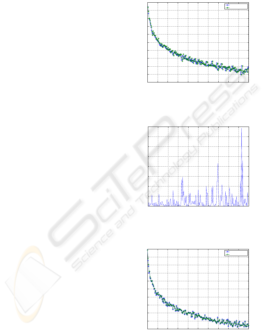
4 RESULTS
The results of the Grey prediction are shown in Fig.
2 which is a plot of the actual values of received
signal strength and corresponding predicted values.
The Grey model tracks the curve with some error
which is shown in Fig. 3. The Grey model does not
predict large variations in the input data. However, to
compensate it we use fuzzy parameters and fine-tune
it with evolutionary algorithms. The parameters
tuned by the evolutionary algorithms are a
ij
, b
ij
and w
i
to minimise the objective function shown
in the Eq. 16. Further, the simulation serves two
purposes: first, to help us decide which evolutionary
algorithm best suits our problem and second to see
the performance of our prediction methodology with
the two evolutionary algorithms and the self tuning
algorithm proposed in (Nomura et al., 1992).
4.1 Comparison on Evolutionary
Algorithms
The prediction methodologies explained in the sec-
tions uses fuzzy parameters which are fined tuned by
evolutionary algorithms. For the experimental setup,
both the genetic algorithm approach and the particle
swarm optimisation approach was used to minimise
the error from the prediction model. Using the Grey
model for prediction of signal strength caused some
errors. The compensated models for the genetic al-
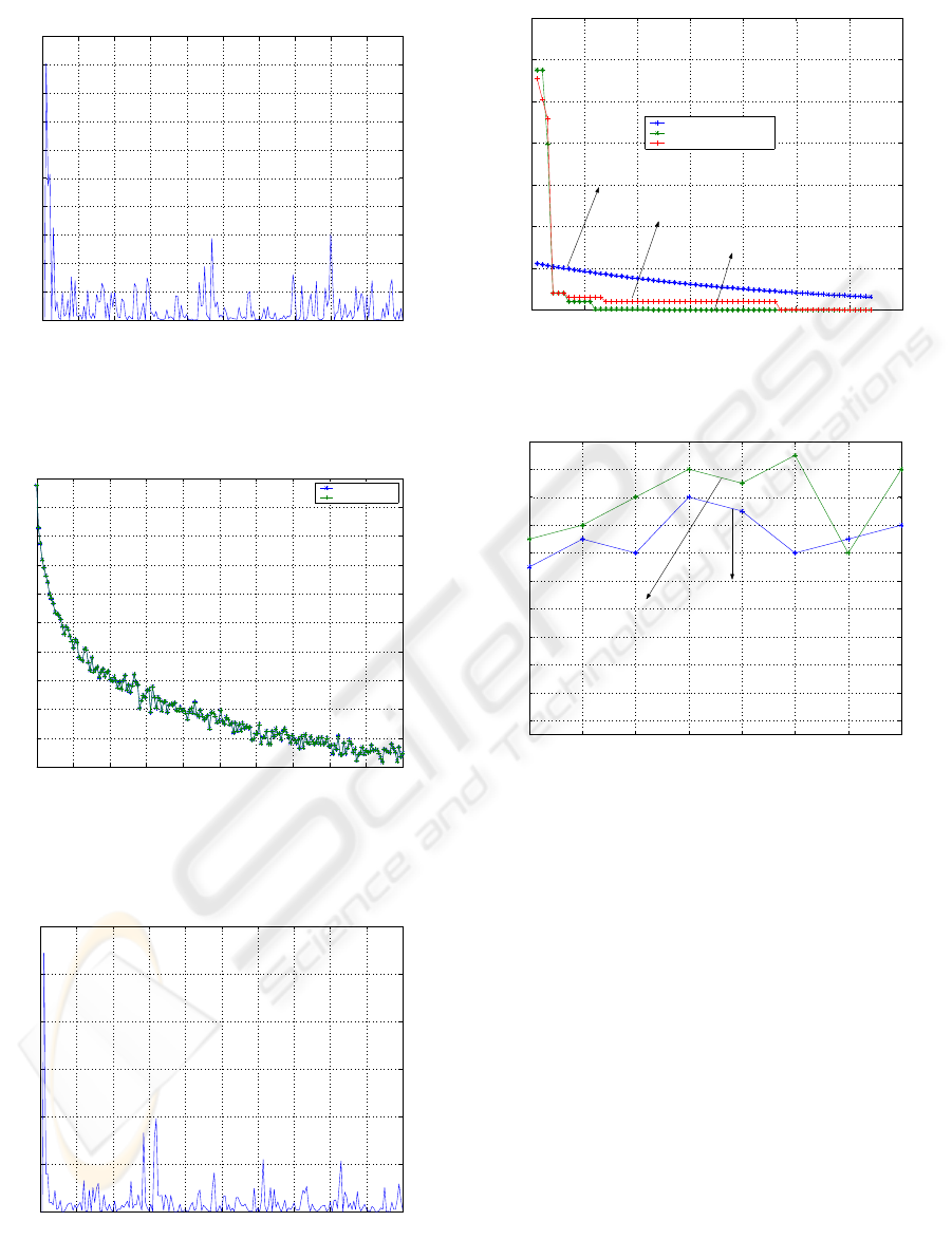
gorithm and PSO are plotted in Fig. 4 and Fig. 5
respectively. We also plotted the absolute errors for
both the models as shown in Fig. 6 and Fig. 7 respec-
tively. Fig. 8 shows the convergence of self-tuning
algorithm, PSO and Genetic algorithms. With our
above hybrid model, it is observed that the PSO has
a better performance than the GA and the self-tuning
algorithm. The fuzzy parameters tuned using the self-
tuning algorithm works with a learning constant set to
the parameters initially, which reduces the error with
every iteration. The self-tuning algorithm takes a very
long time to converge to the minimum value set.
The algorithms were run several times and in 90%
of the cases the PSO converged faster than the ge-
netic algorithm. The PSO reaches the desired fitness
value in lesser iterations than the GA. This is mainly
due the population size chosen initially. The Fig. 9
shows the convergence for the two evolutionary algo-
rithms for several runs. In our experiment, for both
PSO and GA based algorithms the hybrid technique
performs very well giving very minute errors. The
GA was not able to reach the optimum in any of the
experiments in comparison to PSO. This is probably
due to the fairly small population size in the GA. On
the other hand settings of the velocity factors mainly
0 20 40 60 80 100 120 140 160 180 200
−65
−60
−55
−50
−45
−40
−35
−30
−25
−20
−15
Distance
Signal Strength in db
Predicted value
actual value
Figure 2: The received signal strength tracked by the Grey
model.
0 20 40 60 80 100 120 140 160 180 200
0
0.02
0.04
0.06
0.08
0.1
0.12
0.14
0.16
Distance D/d
Signal Strength in dB
Figure 3: The Absolute error from the Grey model.
0 20 40 60 80 100 120 140 160 180 200
−40
−35
−30
−25
−20
−15
−10
−5
0
5
10
Distance d
Signal strength dB
After error compensation using the GA model
Predicted value
actual value
Figure 4: The received signal strength tracked by the Ge-
netic Algorithm model.
OPTIMISATION OF HANDOFF PERFORMANCE IN WIRELESS NETWORKS USING EVOLUTIONARY
ALGORITHMS
115
0 20 40 60 80 100 120 140 160 180 200
0
0.001
0.002
0.003
0.004
0.005
0.006
0.007
0.008
0.009
0.01
Distance D/d
Signal Strength in dB
Absolute error in GA
Figure 5: The absolute error after compensation by the Ge-
netic Algorithm model.
0 20 40 60 80 100 120 140 160 180 200
−40
−35
−30
−25
−20
−15
−10
−5
0
5
10
Distance d
Signal strength dB
After error compensation using the PSO model
Predicted value
actual value
Figure 6: The received signal strength tracked by the PSO
model.
0 20 40 60 80 100 120 140 160 180 200
0
0.5
1
1.5
2
2.5
3
x 10
−5
Distance D/d
Signal Strength in dB
Absolute error in PSO
Figure 7: The absolute error after compensation by the PSO
model.
0 10 20 30 40 50 60 70
0
0.1
0.2
0.3
0.4
0.5
0.6
0.7
Iterations
MSE
MSE vs iteration
Self tuning Algorithm
Particle swarm optimisation
Genetic Algorithm
Self tuning Algorithm
Genetic Algorithm
Particle swarm optimisation
Figure 8: The outputs of the GA, PSO and the self-tuning
algorithm.
1 2 3 4 5 6 7 8
0
2
4
6
8
10
12
14
16
18
20
Runs
Fitness
Fitness vs runs
Genetic algorithm
Particle swarm optimisation
Figure 9: The comparison on fitness values for several runs
for PSO and GA.
determine the performance of the PSO. Also, previ-
ous research by authors of (James Kennedy and R.C.,
2001) shows that PSO is not sensitive to population
size. We conclude that the compensation by PSO
seems to be much better than the GA due to the ve-
locity factor involved in the PSO.
5 CONCLUSION
In this paper, a hybrid prediction model based on
the particle swarm optimisation and genetic algorithm
was proposed. Here, we compared the self-tuning
algorithm along with the PSO and GA. We have
discussed the application of evolutionary computing
technique to find the optimum way of reducing the
error by fine tuning it with fuzzy parameters and evo-
lutionary algorithms. The Grey model was used as the
prediction methodology and errors were compensated
ICETE 2005 - WIRELESS COMMUNICATION SYSTEMS AND NETWORKS
116

by the evolutionary techniques proposed. Our algo-
rithm showed a better accuracy in comparison to any
of the existing prediction methodologies. We have
compared the two evolutionary techniques namely the
genetic algorithms and particle swarm optimisation
in terms of convergence. Each of these search tech-
niques on its own has its specific problem dependent
strengths and weaknesses. GA’s, for instance, are
widely applicable and particularly powerful when do-
main knowledge can be incorporated in the operator
design. However, particle swarm optimisation (PSO)
can achieve clearly superior results in many instances
of numerical optimisation, but there is no general su-
periority compared to GA’s.
We can conclude that, to our context problem the
GA did not perform as well as the PSO because a GA
needs a bigger population size. The GA algorithm
works better for more individuals (increased popu-
lation size) to find a good solution that it can mu-
tate. The PSO, on the other hand, has particles which
are there ‘forever’ and can locate better results in the
search space. Thus, our proposed prediction tech-
nique performs best with particle swarm optimisation
rather than the traditional Genetic algorithm. In future
work, we shall attempt to improve the performance of
the evolutionary algorithms so that they converge at a
faster rate.
ACKNOWLEDGMENTS
The authors wish to thank the Australian Telecommu-
nications Co-operative Research Centre (ATcrc) for
their financial support of this project. We would also
like to thank the people of the CATT Centre, Robert
Suryasaputra and Dr. John Murphy for their helpful
suggestions.
REFERENCES
Chellappa, R., Jennings, A., and Shenoy, N. (2003). Route
discovery and reconstruction in mobile ad hoe net-
works. In Networks, 2003. ICON2003. The 11th IEEE
International Conference on, pages 549–554.
Deng, J. L. (1989). Introduction to grey system theory. J.
Grey Syst., 1(1):1–24.
Hwang, C.-L. (2004). A novel takagi-sugeno-based robust
adaptive fuzzy sliding-mode controller. Fuzzy Sys-
tems, IEEE Transactions on, 12(5):676–687.
James Kennedy, J. and R.C., E. (2001). Swarm Intelligence.
Morgan Kaufmann Publishers, san Francisco,CA.
Janacek, G. and Swift, L. (1993). Time series Forecast-
ing, Simulation, Applications. Ellis Horwood, Great
Britain.
Krink, T., Vesterstrom, J., and Riget, J. (2002). Particle
swarm optimisation with spatial particle extension. In
Evolutionary Computation, 2002. CEC ’02. Proceed-
ings of the 2002 Congress on, volume 2, pages 1474–
1479.
Kung, C.-C. and Lai, W.-C. (1999). ga - based design of a
region-wise fuzzy sliding mode controller. In Electri-
cal and Computer Engineering, 1999 IEEE Canadian
Conference on, volume 2, pages 971–976 vol.2.
Maeda, M. and Miyajima, H. (2002). Constructive
methods of fuzzy rules for function approxima-
tion. In IThe 2002 International Technical Confer-
ence On Circuits/Systems,Computers and Communi-
cations, Phuket, Thailand.
Man, K. F. K. F. (1999). Genetic algorithms : con-
cepts and designs. 1951- Date: London ;New York
:Springer,c1999.
Nomura, H., Hayashi, I., and Wakami, N. (8-12 March
1992). A learning method of fuzzy inference rules by
descent method. Fuzzy Systems, 1992., IEEE Interna-
tional Conference on, pages 203 – 210.
Rappaport, T. (1996). Wireless communications Principles
and practice,3rd Ed. Prentice Hall publication, New
Jersey.
Sheu, S. and Wu, C. (2000). Using grey prediction theory
to reduce handoff overhead in cellular communication
systems. Personal, Indoor and Mobile Radio Commu-
nications, 2000. PIMRC 2000. The 11th IEEE Inter-
national Symposium on, 2(6):782 786.
Shi, Y. and Mizumoto, M. (Aug. 1999). A learning algo-
rithm for tuning fuzzy inference rules. Fuzzy Sys-
tems Conference Proceedings, 1999. FUZZ-IEEE ’99.
1999 IEEE International, 1:378 – 382.
Su, W., Lee, S. J., and Gerla, M. (2000). Mobility prediction
in wireless networks. In MILCOM 2000, 21st Cen-
tury Military Communications Conference Proceed-
ings, volume 1, pages 491–495.
Tran, H. and Harris, R. (2003). Solving qos multicast rout-
ing with genetic algorithms. In Information, Commu-
nications and Signal Processing, 2003 and the Fourth
Pacific Rim Conference on Multimedia. Proceedings
of the 2003 Joint Conference of the Fourth Interna-
tional Conference on, volume 3, pages 1944–1948
vol.3.
Tripathi, N., Reed, J., and VanLandinoham, H. (Dec.1998).
Handoff in cellular systems. IEEE Personal Commu-
nications, 5(6):26–37.
Venkatachalaiah, S., Harris, R., and Murphy, J. (2004). Im-
proving handoff in wireless networks using grey and
particle swarm optimisation. In CCCT, volume 5,
pages 368–373.
Wu, J.-R. and Ouhyoung, M. (1995). A 3d tracking ex-
periment on latency and its compensation methods in
virtual environments. In Proceedings of the 8th an-
nual ACM symposium on User interface and software
technology, pages 41–49. ACM Press.
OPTIMISATION OF HANDOFF PERFORMANCE IN WIRELESS NETWORKS USING EVOLUTIONARY
ALGORITHMS
117
