
USING RELEVANT SETS FOR OPTIMIZING XML INDEXES
Paz Biber, Ehud Gudes
Dep. of comp. science, The Open U., Rabotzki 108, Ra'annana, Israel
Keywords: Local bisimulation, Relevant set, A(k)-Index, Partial order relation.
Abstract: Local bisimilarity has been proposed as an approximate structural summary for XML and other semi-
structured databases. Approximate structural summary, such as A(k)-Index and D(k)-Index, reduce the
index's size (and therefore reduce query evaluation time) by compromising on the long path queries. We
introduce the A(k)-Simplified and the A(k)-Relevant, approximate structural summaries for graph
documents in general, and for XML in particular. Like A(k)-Index and D(k)-Index, our indexes are based on
local bisimilarity, however, unlike the previous indexes, they support the removal of non-relevant nodes.
We also describe a way to eliminate false drops that might occur due to nodes removal. Our experiments
shows that A(k)-Simplified and A(k)-Relevant are much smaller then A(k)-Index, and give accurate results
with better performance, for short relevant path queries.
1 INTRODUCTION
XML (eXtensible Markup Language) has rapidly
become the data representation language of choice
for information exchange on the web (Bray, T., et
al.), (Busse, R., et al, 2001). XML document is a
semi-structured database (Buneman, P., et al, 1997),
(Li, Q. and Moon, B., 2001) , i.e. can be described as
a directed graph. In Figure 1 we see an example of a
graph representing a semi structured database. As
with relational databases, evaluating queries using
only the original database can be very costly in
terms of time and resources needed. Clearly, an
index is needed for an efficient evaluation. Several
types of indexes were suggested, such as connection
indexes, which are designed to support ancestor-
descendent connection, like HOPI (Schenkel, R. et
al., 2004), but most of the indexes proposed are
based on structure summary of the document.
Existing structure summaries are based on NFA to
DFA transition like Strong DataGuide (Goldman, R.
and Widom, J., 1997), graph index with hash tree to
support common prefixes, like APEX (Chung, C. W.
et al., 2002), and bisimilarity based summaries like
1-Index (Milo, T. and Suciu, D., 1999), (Kaushik, R.
et al., 2003) , T-Index (Milo, T. and Suciu, D.,
1999), F&B-Index (Kaushik, R. et al., 2002), A(k)-
Index (Kaushik, R. et al.) and D(k)-Index (Qun, C.,
Lim A. and Ong, K. W., 2003).
In this paper we introduce A(k)-Simplified and
A(k)-Relevant – a structure summary of a semi
structured database, based on local bisimilarity,
which supports removing nodes with non relevant
tags (and therefore significantly decreasing the index
size), while saving the document structure, so short
queries can still be answered accurately. The main
assumption our indexes is based upon is that we can
classify the tags into 2 groups: relevant and non
relevant (as mentioned in (Kaushik, R. et al.,
2002),(Qun, C., Lim A. and Ong, K. W., 2003)). By
declaring a tag as a relevant tag we either mean that
the expression paths are built from relevant tags only
– and we have A(k)-Simplified to support query
evaluation, or, we mean that the results
will be
composed of relevant tags only – and we have A(k)-
Relevant to support these queries. The proposed
approximate indexes are much smaller then A(k)-
Index, and therefore give much better processing
time results. Additional contributions in this paper
are:
1. Presenting a method to eliminate false drops in
A(k)-Simplified and A(k)-Relevant (with respect to
A(k)-Index) using partial order. This method
increases the size of the indexes only by a tiny
amount, and uses data saved on a small percent of
the edges.
2. Showing experimentally that A(k)-Simplified and
A(k)-Relevant reduce both the size of the index and
the processing cost (compared to A(k)-Index). We
also examine the indexes behavior when evaluating
queries with length greater then k.
The idea of replacing irrelevant tags with the label
"other", as a method to reduce index size, appeared
13
Biber P. and Gudes E. (2005).
USING RELEVANT SETS FOR OPTIMIZING XML INDEXES.
In Proceedings of the First International Conference on Web Information Systems and Technologies, pages 13-23
DOI: 10.5220/0001229400130023
Copyright
c
SciTePress

already both in (Milo, T. and Suciu, D., 1998) and
(Kaushik, R. et al., 2002). However, both papers do
not elaborate on the algorithmic implications of this
idea, and in the context of A(k)-Index. This
algorithmic elaboration is the main contribution of
this paper (see also section 2).
The rest of the paper is organized as follows: We
review existing work in section 2, then we elaborate
on the data model and other related issues in section
3 – preliminaries. Afterwards we describe A(k)-
Simplified and A(k)-Relevant in section 4, and then
we give a way to remove false drops in section 5.
We then conclude with experimental results (section
6) and further research (section 7).
2 RELATED WORK
In semi-structured databases, indexes are structural
summaries, made to reduce time for query
evaluation. Some of the indexes are approximate,
which means that for some queries, verification is
needed in order to remove false drops (by the term
false drops we mean false positive – some of the
index's results are incorrect). Examples for such
indexes are: Approximate DataGuide (Goldman, R.
and Widom, J., 1999), which is based on Strong
DataGuide in which “similar” nodes are merged,
APEX (Chung, C. W. et al., 2002) – An index that
adjusts its structure using data mining strategies in
order to efficiently evaluate queries with common
suffixes, D(k)-Index (Qun, C., Lim A. and Ong, K.
W., 2003), which uses different local bisimilarity
values in order to emphasize important tags, and
A(k)-Index. In our work we are interested in the
A(k)-Index and local bisimilarity on which it is
based. We say that two nodes are bisimilar if the two
groups of incoming label path are similar. Every
node in a bisimilarity based index is an equivalence
class for the bisimilar relation. The first bisimilarity
based index was 1-Index, which is safe and accurate
but tends to be very large, especially with “complex”
documents. A(k)-Index offers a way to reduce the
index size by relaxing the bisimilarity demand for
having all the incoming label paths, and declaring a
new relation – local bisimilarity. Two nodes are k
local bisimilar, if their two groups of incoming label
paths, not longer than k, are similar. Local
bisimilarity is based on the assumption that long
queries are rare, and therefore we can build a
structure that gives accurate results for short queries,
while in long queries the results are approximate,
and sometimes need verification (i.e. A(k)-Index is
safe). Experiments show that A(k)-Index is much
smaller then 1-Index.
In A(k)-Index both relevant and non-relevant tags
gets the same treatment, because we define one k for
all the index, in D(k)-Index we can emphasize
relevant tags by giving the nodes with the desired
tags different ‘k’ (local similarity) value, however,
in spite the fact that some tags are known to be non
relevant at all, D(k)-Index still includes all the nodes
whether their tags are relevant or not.
As seen in (Kaushik, R. et al., 2002),(Milo, T.
and Suciu, D., 1998) using partial data can improve
evaluation time. The schema in (Milo, T. and Suciu,
D., 1998) is based on simulation and is used for
creating efficient regular path expressions, which
improves DB scanning time. "other" edges are used
as a replacement for unknown tag's edges which
exist in the DB. However, the goal of the data
structure in (Milo, T. and Suciu, D., 1998) differs
from the goal of (Kaushik, R. et al., 2002) and ours.
We use a bisimulation data structure to efficiently
evaluate the query, rather then creating a more
efficient one, both (Kaushik, R. et al., 2002) and us
offer a method to reduce the index size, by replacing
irrelevant tags with the tag "other", and removing
isolated "other" nodes. This method allows an
efficient evaluation of queries based on relevant tags
only. (Kaushik, R. et al., 2002) uses this method to
reduce the F&B index size, but does not give
detailed algorithms for constructing the index and
evaluating the query using "other". We present these
algorithms in depth, especially in the context of
A(k)-Index structure, and exploit the local
bisimulation in treating "other" nodes. A(k)-
Simplified uses this idea and adds a method to
remove "other" node's path, and A(k)-Relevant
exploits local bisimilarity and relaxes the demand
for queries with relevant tags only, by just requiring
a relevant tag at the end of the query and therefore
supports all queries which return relevant data. Both
indexes support the collapse of "other" paths without
introducing false results.
3 PRELIMINARIES
XML or other semi-structured databases are
modeled as a directed, labeled graph G, with each
edge indicating an object-subobject or object-value
relationship. Each node in G has a label, and an OID
(as described in (Papakonstantinou, Y., 1995)), with
simple objects having a distinguished label,
VALUE. In Figure 1 we can see an example of a
semi structured data graph. The id-idref edges are
sketched with dotted line, but in our model, we
consider all the edges in the same manner. Queries
in semi structured databases are based on regular
path expression. Let G be a data graph, and Σ
G
be
WEBIST 2005 - INTERNET COMPUTING
14

the set of labels in G, we define a regular path
expression R as follows: R := L | _ | R.R | (R|R ) |
R*, where L∈ Σ
G
, ‘_’ denotes any label (one label
only), ‘.’ denotes sequence, ‘|’ alternation and ‘*’
denotes repetition. From now on, we will use a
common abbreviation – the sign “*.” will replace
“_*.”. Before explaining the usage of regular path
expressions, we give some formal definitions. A
node path in G is a sequence of nodes, n
1
, n
2
,… n
m
,
such that n
i
∈G, and an edge exists between n
i
and
n
i+1
for 1≤i≤m-1 . A label path is a sequence of
labels l
1
, l
2
,… l
m
. A node path matches a label path if
label(n
i
)=l
i
for 1≤i≤m. We denote L(R) to be the
regular language specified by R, and we say that R
matches a data graph node n if there is a label path
for some word in L(R) that matches a node path
ending in n. Now, the result of evaluating a query R
on a data graph G, is the set of nodes in G that
matches R. for example, the path expression
*.movie.title evaluated on Figure 1 data graph, is all
the movie’s titles.
Each node in the index graph is associated with
an extent, which is the set of nodes in the matching
equivalence class. If an edge exists from a node in
one equivalence class to a node in another
equivalence class, we add the appropriate edge to the
index. We denote the index for data graph G as I
G
.
Evaluating a query, which is a regular path
expression R on I
G
is a union of the extents of index
nodes in I
G
that matches R.
Definition 1. (Safe and Accurate) Let R be a
regular path expression, we say that an index I
G
is
safe if for each node
v∈V
G
, if R matches v, then v is
in the result of evaluating R on I
G
. We say that I
G
is
accurate if for each node
v∈V
G
, R matches v if and
only if
v is in the result of evaluating R on I
G
.
Definition 2. (Reversed Bisimulation) Let G be a
data graph in which the symmetric, binary relation
≈, the reversed bisimulation, is defined as : two
nodes
u and v are bisimilar (u ≈ v), if:
1. u and v have the same label.
2. if u’ is a parent of u, then there is a parent v’ of v,
s.t. u’ ≈ v’, and vice verse.
Definition 3. (Local Bisimulation – k-
Bisimilarity) Let G be a data graph in which the
symmetric, binary relation ≈
k
, the local bisimulation,
is defined inductively: given the local similarity
value k, we define two nodes u and v to be k-
bisimilar (u ≈
k
v) recursively:
1. u ≈
0
v iff u and v have the same label.
2. u ≈
k
v iff u ≈
k-1
v and for every parent u’ of u, there
is a parent v’ of v, s.t. u’ ≈
k-1
v’, and vice verse.
If two nodes are bisimilar then all the incoming
label paths are equal, while if two nodes are k-
bisimilar, then all the incoming label paths not
longer then k, are equal. 1-Index and A(k)-Index are
based on bisimulation and k-bisimilarity
respectively. We note that 1-Index is accurate while
A(k)-Index is safe. In Figure 1 we see an example of
A(0)-Index (label split index), A(1)-Index and 1-
Index for the data graph shown in Figure 1. Each
index node has its extent attached.
A command is the basic instruction that a script
file contains. Some commands require parameters
that further define what the command should do. An
expression is a combination of operators and
arguments that create a result. Expressions can be
used as values in any command. Examples of
expressions include arithmetic, relational
comparisons, and string concatenations.
3.1 The Set L
Normally we can split our DB into relevant and
irrelevant data (with respect to the queries on the
database). For example, in our movie database we
might want to query only movies or actors so
director and director’s name are irrelevant. We split
the database by defining L (L ⊂ Σ
G
) to be the set of
relevant tags in the database. We will see later in
this paper that by exploiting the existence of L, we
can reduce the index size and query evaluation time
significantly. By defining L, we should consider two
types of queries containing relevant tags:
1. Relevant queries. Queries built only on relevant
tags. i.e. the query is a regular path expression R,
Figure 1: Semi structured database represented as a graph, 1-Index and A(k)-Index
(b) A(0)-Index (c) A(1)-Index (d) 1-Index (a) Database
1
MovieDB
A
A
2
4
N
3
N
5
D
M
T
N
D
N
M
T
6
8
7
9
10
11
12
13
1
MovieDB
A
A
2
4
N
3
N
5
D
M
T
N
D
N
M
T
6
8
7
9
10
11
12
13
1
MovieDB
A
A
2
4
3,5
N M
T
D
N
M
8
6,10
7,11
12
9,13
1
MovieDB
A
A
2
4
3,5
N M
T
D
N
M
8
6,10
7,11
12
9,13
1
MovieDB
A
2,4
N
D
M
T
8,12
6,10
3, 5, 7,11
9,13
1
MovieDB
A
2,4
N
D
M
T
8,12
6,10
3, 5, 7,11
9,13
MovieDB
A
A
N
“actor1”
N
“actor2”
D
M
T
N
“director1”
“movie2”
D
N
“director2”
M
T
“movie1”
1
2
4
35
6
8
7
9
10
11
12
13
MovieDB
A
A
N
“actor1”
N
“actor2”
D
M
T
N
“director1”
“movie2”
D
N
“director2”
M
T
“movie1”
1
2
4
35
6
8
7
9
10
11
12
13
USING RELEVANT SETS FOR OPTIMIZING XML INDEXES
15

R=r
1
.r
2
. … r
n
, and for i=1,…,n-1, r
i
∈L ∪ {‘*’,
(r
i
1
|r
i
2
)}, r
n
∈L
2. Relevant end queries. Queries that end with a
relevant tag. This means we have relevant tags as
our results, but irrelevant tags can be a part of the
queries. We define those queries as a regular path
expression R, R=r
1
.r
2
. … r
n
, and for i=1,…,n-1,
r
i
∈V
G
∪ {‘*’, (r
i
1
|r
i
2
)}, r
n
∈L.
The symbol “_” was not mentioned, but since we
are using a relevant set, it can be used in queries
only in order to replace a relevant tag.
In this paper we will propose 2 indexes: A(k)-
Simplified and A(k)-Relevant. These indexes exploit
the existent of L in order to reduce index size and
query evaluation time. A(k)-Simplified is very
efficient when evaluating queries from the first type
(relevant tags only), while A(k)-Relevant supports
both type of queries, and is preferred when dealing
with queries which contains irrelevant tags along the
path. A(k)-Simplified and A(k)-Relevant are very
efficient when L is defined, and the queries comply
with one of the two types. If this is not the case,
using these indexes may result in false drops. The
term 'relevant' will be used both when discussing
tags and nodes with relevant tags. The meaning will
be clear from the context.
4 A(K)-SIMPLIFIED AND A(K)-
RELEVANT
4.1 Introduction to A(k)-Simplified
and A(k)-Relevant
A(k)-Simplified index is based on k-bisimilarity by
the fact that we preserve all the incoming paths with
length less or equal to k. furthermore, giving the set
L, each tag in A(k)-Simplified is either from L or
“other”. A(k)-Simplified is built by replacing all the
irrelevant tags by the tag “other”, and then replacing
an “other” tree with one “other” node. A(k)-
Relevant is also based on k-bisimilarity, but in this
index, besides the relevant tags and the tag “other”,
we preserve the tags of nodes that have a relevant
descendant in distance not greater than k (we will
elaborate later in this section). A(k)-Simplified is the
index which results from the following 4 steps (see
also section 4.2): Replacing all the irrelevant tags
with the tag “other”, Removing all the nodes with
tag “other” with no relevant descendent node,
Applying the A(k)-Index building algorithm,
Replacing every “other” node tree with one “other”
node. Before building A(k)-Relevant there are 2
important issues that should be considered:
1. Like A(k)-Simplified, if there is an “other” node
from which we cannot reach a relevant tag node,
then the “other” node can be removed.
2. A(k)-Index properties suggest that two data graph
nodes
u, v will be in the same extent if all the
incoming label paths with length ≤ k are the same,
and there is a node with tag T which is k+1 steps
from
u and which is not matched by any node
with tag T and k+1 steps from
v. Since A(k)-
Relevant supports queries that end with relevant
tag nodes, we can conclude that there is no need
to preserve the tag of irrelevant nodes with
distance k+1 or more from a relevant node.
Building A(k)-Relevant is quite similar to
building A(k)-Simplified, with a small modification
in the first step: Replacing all the irrelevant tags of
nodes with no relevant tag descendent within
distance less or equal to k with the tag “other”.
A(k)-Simplified and A(k)-Relevant have the
following properties (w.r.t A(k)-Index (Kaushik, R.
et al.), (Qun, C., Lim A. and Ong, K. W., 2003)) :
1. For relevant tags, which are our main (and usually
all) interest, A(k)-Relevant keeps all paths with
length ≤ k (and therefore accurate for those
queries). Using false drops removal, A(k)-
Simplified is also accurate for relevant queries
with length ≤ k.
2. A(k)-Simplified and A(k)-Relevant are safe.
For k values large enough, A(k)-Simplified and
A(k)-Relevant do not change (they have a steady
structure) and they can be considered as 1-Index
with relevant support.
4.2 Construction Algorithms
We first describe the A(k)-Simplified construction
algorithm and then the modifications needed for
building A(k)-Relevant. The construction algorithm
has 4 steps:
1. Collapse – replacing irrelevant tags with the tag
“other”, and removing irrelevant nodes which
have no relevant descendent.
2. A(k)-Index – creating an index structure where k-
bisimilar nodes are combined to the same extent.
3. MaxOtherPath – marking the “other” trees.
4. Replacing other trees – replacing the trees
marked in step 3 by one “other” node.
Algorithm 1: Collapse
Input: The inversed data graph G’=(V,E).
Output: The data graph G with irrelevant tags
replaced with the tag “other”, and irrelevant nodes
with no relevant descendent removed.
1. Empty (Q)
2. for each vertex v∈V(G) do
WEBIST 2005 - INTERNET COMPUTING
16

3. If v∈L (Relevant) then Distance(v) = 0;
Status(v) = "Visited"; Enqueue(Q,v)
4. Else Distance(v) = ∞; Status(v) = "Not
Visited"; Label(v) = "other"
5. While Q is not Empty
6. u = head(Q)
7. for each s son of u do
8. if Status(s) = "Not Visited" then
Status(s) = "Visited"; Distance(s) = Distance(u)
+ 1; Enqueue(Q,s)
9. Dequeue(Q)
10. Status(u) = "Finished"
11.Remove all vertices with Distance = ∞ and
Reverse G’ back to G
We can see the collapse running example in
Figure 2. We remark that the input is G’ (G
reversed) because the distance is calculated from the
descendents to their parents. We will also remark
that in step 8 we save the distance from a irrelevant
node to a relevant node. This is not important here
(in A(k)-Simplified we are only interested to know
whether it is ∞ distance (no path) or not). We will
use this parameter later, when we describe A(k)-
Relevant. The algorithm is based on BFS with some
modifications – we traverse G’ – the reversed graph
and initialize the next node queue with all the
relevant nodes (the grey nodes in Figure 2 will
become clearer when we describe A(k)-Relevant)
As stated earlier, the next step is applying A(k)-
Index to Collapse’s result. The algorithm is
described in (Kaushik, R. et al.). The third step is
MaxOtherPath - this algorithm is based on depth
first search, where for each “other” node we
encounter – we either relate it to the current path (if
exist) or start a new path. The motivation is to mark
"other" nodes trees before replacing each one with a
single node.
Algorithm 2: MaxOtherPath
Input: The result of the second step (A(k)-Index) –
the index graph G.
Output: The index graph G with each “other” node
related to an "other" tree. Each "other" tree has a set
of all incoming and outgoing edges.
1. Global-Current-Tree = 0
2. For each vertex u∈V(G) Visited(u) = Never;
Path(u) = Global-Current- Tree
3. MaxOtherPath-DFS-Visit(root, False, 0)
MaxOtherPath-DFS-Visit
(u, Path-Indication,
Current-Tree)
1. Visited(u) = Visited
2. if u∈L (i.e. Relevant) then Tree -Indication =
False
3. Else
4. If Tree -Indication = False then Path-
Indication = True; Global-Current-Tree =
Global-Current-Tree +1; Current-Tree =
Path(u) = Global-Current-Tree
5. Else Path(u) = Current-Tree
6. For each v∈Son(u)
7. If Visited(v) = Never then
8. MaxOtherPath-DFS-Visit(v, Path-Indication,
Current-Tree)
9. For each path found – walk through the nodes
and for every edge not part of the path add it to
incoming set or outgoing set according to the
edge origin.
We can see an example of MaxOtherPath in
Figure 3. The last step of the construction algorithm,
is replacing each “other” nodes tree by one “other”
node. This is done simply by removing all the
“other” nodes and their edges and replacing them
with one node with tag “other”. For every incoming
and outgoing edge we saved in step 9 in
MaxOtherPath, we add the appropriate edge to our
new node (see
Figure 3d). Note that if instead of
replacing every “other” tree, we replace all the
“other” nodes with one node, we may add many
false drops, and this may cause a lot of verifications
when we process the queries, and therefore
substantially increase time for evaluating the
queries. We will also note that self edges will be
created when we have 2 (or more) “other” paths
(paths built on “other” nodes only) from one “other”
Figure 2: collapse algorithm (k=2): (a) the original data graph (relevant notes are black, irrelevant nodes –
white) (b) the reversed graph, (c)-(e) three passes of steps 12-18, (f) result
(a)
original
(b) the
inversed
(c) after first
pass
(d) after
second pass
(e) after
third pass
(f) collapse
result
0
1
∞
2
0
∞
1
0
∞
∞
0
1
∞
∞
0
∞
1
0
∞
∞
0
1
3
2
0
∞
1
0
3
∞
USING RELEVANT SETS FOR OPTIMIZING XML INDEXES
17

node to another. For now, self edges can be omitted;
we will discuss this in the next section – removing
false drops.
Until now we discussed A(k)-Simplified
building algorithm. As we have already seen, the
difference between A(k)-Simplified and A(k)-
Relevant is that the former replaces the tag of all the
irrelevant nodes with the tag “other”, while the latter
only replaces the tag of irrelevant nodes with distant
relevant descendent (distance > k). In order to
achieve this, we have to modify the first step
(collapse). The modifications are: k will be added to
the input for the algorithm, and instead of replacing
all the irrelevant nodes, we will replace only those
nodes which have distance > k. In Figure 2f, we
marked with gray dots the irrelevant nodes which
will not be tagged as “other”. If the data graph is
G=(V,E), the total constructing time is O(k
⋅
|E|)
(A(k)-Index time complexity). In more details, we
have the time complexity O(|E|) for collapse (BFS
complexity), O(k
⋅
|E|) (Kaushik, R. et al.) for A(k)-
Index, O(|E|) for MaxOtherPath (DFS complexity)
and O(|E|) for replacing other trees (removing
irrelevant nodes, and restoring all the effected
edges).
Theorem 1. A(k)-Simplified is safe for l
≤
k
relevant queries. A(k)-Relevant is safe and accurate
for l
≤
k relevant end queries.
Proof. Obvious from the indexes definitions.
5 REMOVING FALSE DROPS
As mentioned earlier, replacing the “other” trees
may result in increasing number of false drops (w.r.t.
A(k)-Index). In
Figure 4 we can see that replacing
the irrelevant tree increases the number of false
drops in A(k)-Simplified for paths with length < k
(in
Figure 4b the dotted line shows the path which
does not exist in the original data graph). A(k)-
Relevant is accurate for short relevant end queries,
however, in
Figure 4 we see an example where for
path longer than k, A(k)-Relevant adds false drops
which are not returned by a lookup in the A(k)-
Index. In
Figure 4c the dotted line marks the result
of the query R.A.*.B. In
Figure 4d we see the result
of this query on A(4)-Relevant, which includes one
false drop.
The reason for increasing number of false drops
w.r.t. A(k)-Index is that we replace the “other” trees
with one node and add paths which do not exist in
the original graph. From these observations we see
that removing invalid paths involving “other” nodes
can reduce the number of false drops for A(k)-
Simplified (for queries in any length) and for A(k)-
Relevant (query’s length > k). In this section we will
present a method to remove these invalid paths. For
each “other” tree replaced by one node, we mark the
location of every incoming and outgoing edge, and
use these marks in query calculation. We now
describe a way to mark the edges using a partial
order relation.
5.1 Partial Order Relation
The intuition for using partial order relation is the
observation that it stands for the relation
"descendent of" between 2 nodes in an "other" tree
discovered by collapse, and therefore, by keeping
the partial order relation between the nodes we can
reconstruct the original paths, and remove the false
paths.
We save the location of every node in each
“other” tree
in the following way: p
1
;p
2
;…;p
n
;d
(n>0). p
i
represents the path from the root to the
node, d represents the node’s depth. By the term
“other” tree we mean the sequence of “other” nodes
discovered during the MaxOtherPath algorithm. The
meaning of p
i
is: We mark the first “other” node
discovered in the “other” path (the path’s root) by ;1
which stands for depth 1 (d=1, i=0). Assuming we
are in an “other” node
u which is marked with
p
1
;p
2
;…;p
k
;d then:
1. if
u does not have an “other” child node there
is nothing to do.
2. If
u has exactly one “other” child node, it will
be marked with p
1
;p
2
;…;p
n
;d+1
3. if u has k>1 “other” children nodes, their mark
will be: p
1
;p
2
;…;p
k
;d;1;d+1, ...,
Figure 3: MaxOtherPath and “other” tree replacement algorithm
(a) original
data graph
(b) partial results
of MaxOtherPath
(c) MaxOtherPath
result
(d) Replacing “other”
tree with one node
WEBIST 2005 - INTERNET COMPUTING
18

p
1
;p
2
;…;p
k
;d;k;d+1. (we concatenate m;d+1 for
u’s m rightmost “other” child).
We can now define our partial order relation.
Assume that A=a
1
;a
2
;…;a
na
;d
a
, B=b
1
;b
2
;…;b
nb
;d
b
(A,B represent two locations in an “other” path), we
define the relation “≤’”: A≤’B if a
1
;a
2
;…;a
na
⊂
b
1
;b
2
;…;b
nb
(a
1
;a
2
;…;a
na
is not equal but is a prefix
of b
1
;b
2
;…;b
nb
) or if a
1
;a
2
;…;a
na
=b
1
;b
2
;…;b
nb
and
d
a
≤d
b
. This is a partial order relation – it is reflexive,
antisymetric and transitive. We will see later on, that
given 2 nodes u,v in an “other” tree there are three
possibilities, either there is a path from u to v (which
translates to Mark(u)≤’Mark(v)), a path from v to u
(Mark(v)≤’Mark(u)) or there is no path at all (no
relation between the Mark(u) and Mark(v)). After
defining the relation ≤’, we should mark the “other”
nodes and take this mark into consideration when
querying the index. In MaxOtherPath, when we
traverse an “other” tree we keep two parameters:
trail and depth, and we mark each node with
trail;depth, the trail corresponds to p
1
,p
2
,..,p
k
and the
depth corresponds to d. when replacing the "other"
nodes tree with one “other” node we give each
ingoing/outgoing edge two values: ingoing mark and
outgoing mark. If the origin of the edge is from a
relevant node (not an “other” node) its origin mark
will be null, else, its origin mark will be the “other”
node’s mark. We treat the node’s destination mark
with a same manner. In
Figure 5 we can see an
example of how we mark each node in the “other”
tree, and how we use those marks to mark the origin
and destination of the appropriate edges.
5.2 Handling Self Edges
Both in A(k)-Simplified and A(k)-Relevant
construction algorithms, self edges could have
been formed when there where 2 (or more) “other”
paths (paths built on “other” nodes only) from one
“other” node to another. Those self edges were
removed because they did not contribute to query
analysis. However, when we add the false drops
treatment, self edges play an important role. More
information regarding self edges and self edges
removal is given in (Biber, P. and Gudes, E., 2005).
Theorem 2. False drops removal eliminates the
invalid paths formed when “other” tree is replaced
by one “other” node.
Proof. In order to show that no invalid path is
added, we will see that there is a path from a node u
to a node v (u and v are both a part of the same
“other” tree, as found by MaxOtherPath) if and only
if Mark(u)≤’Mark(v). if u is an ancestor of v, then
v’s trail is either equal to u’s or has u’s mark as its
prefix – either way Mark(u)≤’Mark(v). The
implication holds also in the opposite direction,
since if Mark(u) ≤’ Mark(v) it means that either v’s
trail is equal to u’s and v’s depth is greater then u’s
or v’s trail has u’s mark as its prefix.
€
From the A(k)-Index and the false drops removal
properties we get the following:
Corollary. When using false drops removal,
A(k)-Simplified is accurate for short relevant
queries, and A(k)-Relevant has less false drops for
l>k relevant end queries.
5.3 Querying the Indexes
Without false drops treatment, the way to compute a
query is equal to the one described in (Kaushik, R.
et al.). In
Figure 6a we can see an example of an
index (it can be Relevant or Simplified), a DFA that
matches the query *.A.B (
Figure 6b), and the results
of the index scan (
Figure 6c) without taking the
marks into consideration. The returned set is the
extent of the index nodes that get an accepting state
(state 3, marked with an arrow). In order to take
advantage of the false drops removal's markings
added to the index, the scanning must consider two
A
B
B
A
C
A
B
C
A
(a)
(b)
A
O
A
A
A
(c)
R
C
A
C
C
C
C
C
B
C
C
C
C
C
B
(d)
R
A
O
C
C
C
C
B
C
C
C
C
B
Figure 4: false drops in A(k)-Simplified and A(k)-Relevant: (a) Original data graph (which is equal to A(3)-
Index). L={A}. (b)
The appropriate A(3)-Simplified. The dotted line represents a path which does not exist in A(3)-
Index (c) Original data graph
(which is equal to A(4)-Index), L={R,A}. The dotted line represents the results of the query R.A.*.B (d) The appropriate A(4)-
Relevant. The dotted line represents the result of the same query on the index (the left B node is a false drop)
USING RELEVANT SETS FOR OPTIMIZING XML INDEXES
19

factors: the edges marking and the self edges. In
Figure 6d we can see the results of the same query
evaluated with marks. In
Figure 4c when the nodes
C6, C7, C1 were translated to “other” nodes, they
got the marking: ;1, ;1;1;2 and ;1;2;2 respectively,
so in
Figure 4d the edge between A and O has a
destination mark 1;1;2 , the edge from O to C2 has
an origin mark 1;1;2 and the edge from O to C8
an origin mark 1;2;2. Now, since 1;1;2 has no ≤’
relation with 1;2;2 when we process the query
R.A.*.B and enter the “other” node from A, we will
not be able to go to C8 and the false drop will be
removed.
6 EXPERIMENTAL STUDY
In this section we present the results of the
conducted experiments. This section layout is as
follows: first we give some background regarding
queries, the cost model, the selection of the relevant
set L and the databases used in the experiments, next
we examine the indexes size and the increase of size
due to false drops removal, afterwards we compare
the time needed to scan the indexes when processing
queries and in the last section we examine the
number of false drops.
6.1 Experimental Framework
Query classification
In our experiments we use a slightly different
classification than the one presented in (Kaushik, R.
et al.). We split the queries into 3 groups:
• Short queries which are queries built on labels
only – for example L
1
.L
2
.L
3
. It is clear that for
short and - relevant or relevant end query -
A(k)-Simplified with false drops removal and
A(k)-Relevant (respectively) are accurate.
• Simple queries which are queries that have
only one “*” located at the beginning of the
queries – for example *.L
1
.L
2
. although when
processing these queries we use paths longer
then k, it can be easily shown that the indexes
are still accurate.
• Complex queries which have more then one
“*” or only one “*” but not as the query’s
starting label. When processing these queries
all of the indexes (including A(k)-Index) may
return false drops, so verification might be
needed.
The experiments results include false drops
verification (whenever it is need). As expected,
verification is needed for complex queries, or when
k is very small.
The cost model
We will use the cost model offered in (Kaushik, R.
et al.). The cost of evaluating a query is the number
of nodes visited in the index during automaton
execution plus the number of nodes visited in the
DB during false drops verification. Note that for
precise queries no verification is needed. The graph
size is calculated as the sum of the graph nodes and
edges.
Selecting the relevant set L
In our experiments, we randomly selected various
sets of relevant labels. There are two ways to
examine the relevant set: the percent of nodes out of
all the data graph nodes which have the relevant tags
or, the percent of the relevant tags out of all the tags
in the database. Our experiments show that the
former is a better measure to predict the indexes size
and accuracy. We also randomly selected the
relevant set, so usually the nodes will be spread all
over the graph, however, in some cases the nodes
will not be spread homogenously so the results can
have some variation, but the experiments always
show a tendency.
The Databases
In the experiments described, two XML databases
were used. The first source is the Internet Movie
Database (IMDB) (The Internet Movie Database
Ltd, “Internet Movie Database”, Available:
http://www.imdb.com) and the second is a synthetic
database generated for performing our experiments.
IMDB was selected because it represents a real life
database with many cycles (Goldman, R. and
Widom, J., 1997). The portion of the database
selected is organized around movie. The synthetic
database is a highly complex database with a lot of
irregularity that allows examining the indexes in
highly irregular conditions, where the index size is
usually very large.
Figure 5: Marking the nodes in the “other” trees, and
the appropriate edges after replacing the trees with
one node
;1
;2
2;2;
2;1;
A
A
;1
A
A
;
2
;2;1;3
;2;2;3
;1
;
;2;1;3
WEBIST 2005 - INTERNET COMPUTING
20
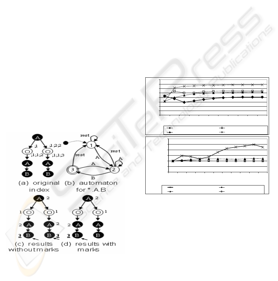
6.2 Index Size
The size of A(k)-Simplified and A(k)-Relevant
increases as k increases but it remains stable
compared to the A(k)-Index’s size. High variation of
the database increases the size of A(k)-Simplified
and A(k)-Relevant (compared to A(k)-Index). The
size of the indexes w.r.t. A(k)-Index is displayed in
Figure 7. The size is calculated for different values
of k, the A(k)-Simplified and A(k)-Relevant are
calculated for different L sets. The size shown in the
graph is the indexes average size over different L
sets, and as we can see A(k)-Simplified is 40%-52%
of A(k)-Index, and A(k)-Relevant is 55%-69% of
A(k)-Index. The increase of size due to false drops
removal (because of self edges addition) is displayed
in the lower figure. As expected, the increase of
A(k)-Relevant’s size is almost zero for small k
values and zero for large k values – since we
preserve the tags of incoming paths with length
smaller or equal to k, the size and complexity of the
“other” paths is reduced and therefore the number of
self edges is also reduced. In A(k)-Simplified the
size increases for larger k, because in the second
step of the building algorithm (A(k)-Index) fewer
“other” nodes merge into one index node, and so in
the fourth step (replacing the “other” trees) more
nodes are replaced and so more self edges are
formed. This trend stops at a certain k value.
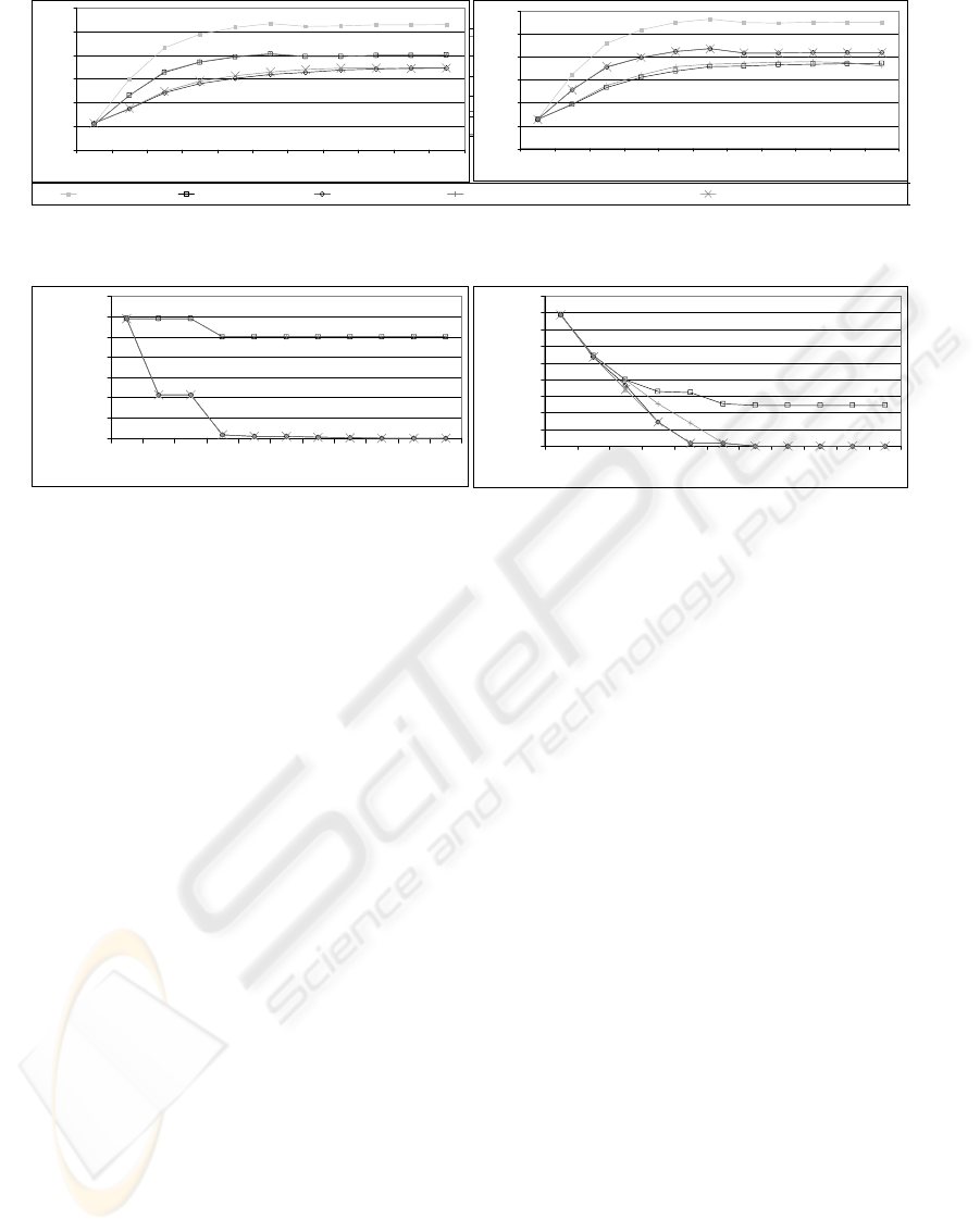
6.3 Query Cost
Figure 8 shows the cost of evaluating various
queries. As expected, the queries evaluation cost for
A(k)-Simplified and A(k)-Relevant with or without
false drops removal is much smaller then evaluating
the query on A(k)-Index. Also as k reaches a certain
value, the evaluation cost stops growing, since the
indexes reach their stable state. As mentioned
earlier, the result here are the index scanning cost
plus verification cost (when needed). For complex
queries, there is always a need to verify the query
results (for all the queries). Since complex queries,
like simple queries, contain “*” (one or more) the
proportion between the A(k)-Index scanning time to
the A(k)-Simplified and A(k)-Relevant scanning
time remains quite similar to those of the simple
queries evaluation. The important factor here is the
number of false drops which causes costly
verification. Figure 9 displays the percent of false
drops for complex queries. It is clear that A(k)-
Simplified without false drops removal has more
false drops (and therefore has a costly evaluation
time). With false drops removal the number of false
drops in A(k)-Simplified is reduced by an order of
tens of percents. As expected, for A(k)-Relevant the
increase of false drops number (w.r.t. A(k)-Index) is
very small – less then 0.3% in average (actually it is
0% most of the time) – here the false drops removal
is less effective though we can still see a small
improvement in the synthetic database. We can also
see that for relevant end queries, A(k)-Relevant has
much less false drops than A(k)-Simplified, which
explains A(k)-Relevant's better results.
Figure 6: Evaluating query on an index.
Figure 7: The indexes size. In the upper figure -
A
comparison between the indexes and A(k)-
Index. In the
lower figure -
the size increase due to false drops
removal (self edges increase).
0%
10%
20%
30%
40%
50%
60%
70%
80%
012345678910
K
Percent of A(k)-Index
A(k)-Simplified in IMDB A(k)-Relevant in IMDB
A(k)-Simplified in synthetic database A(k)-Relevant in synthetic database
99.00%
99.50%
100.00%
100.50%
101.00%
101.50%
102.00%
012345678910
K
Percent of indexes without
false drops removal
A(k)-Simplified in IMDB A(k)-Relevant in IMDB
A(k)-Simplified in synthetic database A(k)-Relevant in synthetic database
USING RELEVANT SETS FOR OPTIMIZING XML INDEXES
21
7 CONCLUSION AND FUTURE
RESEARCH
A(k)-Simplified and A(k)-Relevant are small,
efficient indexes evolved from A(k)-Index. The
indexes offer a way to reduce index size
significantly when prior knowledge of the relevant
tags exists. Though based on A(k)-Index, A(k)-
Simplified and A(k)-Relevant are flexible, and can
be modified to be based on other structured indexes,
such as 1-Index and D(k)-Index. A(k)-Simplified is
very efficient when queries are known to be based
on relevant tags only, while A(k)-Relevant gives
good results when only the ending tags are known.
Performance examination shows that the indexes
give good results while increasing the number of
false drops by a very small proportion (and usually
do not increase false drops at all). We also offered a
method, based on partial order relation, to eliminate
false drops created by nodes removal, while
increasing the size of the index by no more then
1.5%.
More work is needed to modify existing indexes
for supporting irrelevant node’s removal. It seems
appropriate to adjust bisimulation based indexes to
support exploiting relevant set declaration, and
removing irrelevant nodes. Further work is needed
to make A(k)-Simplified and A(k)-Relevant support
DB functionality such as update, insert and delete.
ACKNOWLEDGEMENT
The Idea for A(k)-Relevant originated from
discussions with Philip Bohannon.
REFERENCES
Bray, T., Paoli, J., Sperberg-McQueen, C.M., Maler, E.
and Yergeau, F. (2004, February 2) "Extensible
Markup Language (XML) 1.0 (Third Edition), W3C
Recommendation", Available:
http://www.w3.org/TR/REC-xml.
Busse, R., Carey, M., Florescu, D., Kersten, M., Schmidt,
A., Mauolescu, I., and Waas, F. (2001, April) "The
XML Benchmark Project", Available:
http://monetdb.cwi.nl/xml/index.html.
Buneman, P., Davidson, S.B., Fernandez, M.F., and Suciu,
D. (1997) 'Adding Structure to Unstructured Data',
Proceedings of ICDT.
Li, Q. and Moon, B. (2001) 'Indexing and Querying XML
Data for Regular Path Expressions', Proceedings of
VLDB.
Derose, S., Maler, E. and Orchard, D. (2001, June 27)
"XML Linking Language (XLink), version 1.0, W3C
Recommendation", Available:
http://www.w3.org/tr/xlink.
Chamberlin, D., Florescu, D. and Robie, J. (2000) 'Quilt:
An XML Query Language for Heterogeneous Data
Sources', Proceedings of WebDB.
Figure 8: Query evaluation cost (on synthetic database). The left figure –
Relevant End queries. The right figure
– Relevant queries
0.00%
20.00%
40.00%
60.00%
80.00%
100.00%
012345678910
Percent of false drops
A(k)-Index A(k)-Simplified A(k)-Relevant A(k)-Simplified with False Drops Removal A(k)-Relevant with False Drops Removal
0
500
1,000
1,500
2,000
2,500
3,000
012345678910
K
Number of nodes scanned
0
500
1,000
1,500
2,000
2,500
3,000
012345678910
K
Number of nodes scanned
Figure 9: False drops in complex queries (on IMDB). The left figure – Relevant End queries. The right figure
– Relevant queries.
0.00%
10.00%
20.00%
30.00%
40.00%
50.00%
60.00%
70.00%
80.00%
90.00%
012345678910
K
Percent of false drops
0.00%
5.00%
10.00%
15.00%
20.00%
25.00%
30.00%
35.00%
012345678910
K
Percent of false drops
WEBIST 2005 - INTERNET COMPUTING
22

Abiteboul, S., Quass, D., McHugh, J., Widom, J. and
Wiener, J. (1997) 'The Lorel Query Language for
Semistructured Data', International Journal on Digital
Libraries, 1(1):68-88.
Clark, J. and Derose, S. (1999, November 16) "XML Path
Language (XPath) Version 1.0, W3C
Recommendation", Available:
http://www.w3.org/TR/xpath.
Deutsch, A., Fernandez, M., Florescu, D., Levy, A., and
Suciu, D. (1999) 'A Query Language for XML',
Proceedings of the Eighth World Wide Web
Conference.
Chamberlin, D., Florescu, D., Robie, J., Simeon, J.
and Stefanescu, M. (2005, February 11) " XQuery 1.0:
An XML Query Language, W3C Working Draft",
Available: http://www.w3.org/TR/xquery.
Schenkel, R., Theobald, A. and Weikum, G., (2004)
'HOPI: An Efficient Connection Index for Complex
XML Document Collections', Proceedings of EDBT.
Goldman, R. and Widom, J. (1997) 'Dataguides: Enabling
Query Formulation and Optimization in
Semistructured Databases', Proceedings of VLDB.
Goldman, R. and Widom, J. (1999) 'Approximate
DataGuides', Proceedings of the workshop on Query
Processing for Semistructured Data and Non-
Standard Data Formats, Pages 436-445.
Chung, C. W., Min, J. K. and Shim, K. (2002), 'APEX:An
Adaptive Path Index for XML Data', Proceedings of
SIGMOD.
Milo, T. and Suciu, D. (1999) 'Index Structures for Path
Expressions', Proceedings of ICDT.
Kaushik, R., Bohannon, P., Naughton, J.F. and Shenoy, P.
(2002) 'Updates for Structure Indexes', Proceedings of
VLDB.
Kaushik, R., Bohannon, P., Naughton, J.F. and Korth, H.F.
(2002) 'Covering Indexes for Branching Path Queries',
Proceedings of ACM SIGMOD.
Kaushik, R., Shenoy, P., Bohannon, P. and Gudes, E.
(2002) 'Exploiting Local Similarity for Efficient
Indexing of Paths in Graph Structured Data',
Proceedings of ICDE.
Qun, C., Lim A. and Ong, K. W. (2003) 'D(k)-Index: An
Adaptive Structural Summary for Graph-Structured
Data', Proceedings of ACM SIGMOD.
Papakonstantinou, Y., Garcia-Molina, H. and Widom, J.
(1995) 'Object Exchange Across Heterogeneous
Information Sources', Proceedings of ICDE.
Abiteboul, S. (1997) 'Query Semi-structured Data',
Proceedings of ICDT.
McHugh, J., Widom, J., Abiteboul, S., Luo, Q. and
Rajamaran, A. (1998) 'Indexing Semistructured Data',
Technical Report, Stanford University.
Henzinger, M., Henzinger, T. and Kopke, P. (1995)
'Computing Simulations on Finite and Infinite Graphs',
Proceedings of FOCS.
Milo, T. and Suciu, D. (1998) 'Optimizing Regular Path
Expressions Using Graph Schemas', Proceedings of
ICDE.
The Internet Movie Database Ltd, "Internet Movie
Database", Available: http://www.imdb.com.
Biber, P. and Gudes, E. (2005) 'Improving Algorithms for
Indexes in XML based Databases', Master's thesis,
The Open University of Israel.
USING RELEVANT SETS FOR OPTIMIZING XML INDEXES
23
