Cognitive Map Merging For Multi-Robot Navigation

Anderson A. Silva

, Esther L. Colombini

and Carlos H. C. Ribeiro

NCROMA Research Group

Computer Science Division

Technological Institute of Aeronautics

Prac¸a Marechal Eduardo Gomes, 50 - Vila das Ac

acias

CEP 12228-900, S

ao Jos

e dos Campos - SP, Brazil

Abstract. In this paper we investigate a map-building strategy based on geomet-

ric and topological information about the environment, acquired through sonar

sensors and odometric actuator. To reduce robot individual exploration needs,

a framework based on multi-robot map acquisition is proposed, where each ro-

bot executes a map building algorithm and performs exploration in the environ-

ment. The current global map is built based on the merging of overlapping re-

gions among the previously cognitive maps. A brief description of the on-going

research and the results obtained is also provided.

1 Introduction

In order to deploy robots in a wide variety of applications, a way to program them

efﬁciently has to be found. The main motivation to the development of this research,

that involves autonomous mobile robots, lies in the possibility of having them working

in an unsupervised way in complex, harsh or dangerous tasks that need interaction with

an unstructured environment.

One of the fundamental problems in mobile robotics is that of exploring an un-

known environment. The main goal of this research is the application of map building

techniques to individual robots interacting with their environment. To perform a repre-

sentation of the world the robot perceives it with its on-board sensors and the acquired

data is processed aiming at extracting the most relevant features of the environment.

To take advantage of multi-robot systems, map merging algorithms are applied to

previously acquired individual maps to represent a global view of the former unknown

environment.

2 Map Building

Robotic mapping addresses the problem of spatial models of physical environments

through mobile robotics [1]. Mobile robot networks can provide a dynamic view of the

scene at relevant locations through cooperative navigation.

In [2], Thrun related a set o factors whose inﬂuence can turn the task of model

acquisition a hard one and that impose practical limitation to learning and use of precise

maps. Among the limitations are:

A. Silva A., L. Colombini E. and H. C. Ribeiro C. (2005).

Cognitive Map Merging For Multi-Robot Navigation.

In Proceedings of the 1st International Workshop on Multi-Agent Robotic Systems, pages 102-111

DOI: 10.5220/0001196801020111

 SciTePress

– Sensorial limitation due to sensors range of actuation limited to regions close to the

robot, requiring the agent to explore the environment to search for global informa-

tion;

– Noise in the sensors that normally affect the reading and have an unknown distrib-

ution;

– The kind of information provided by the sensors is not that one that really matters

to the robot (e.g. camera readings represent only colors, brightness, etc), requiring

the application of algorithms to ﬁlter and extract the desired features of the envi-

ronment;

– Odometry errors that cause imprecision in the robot movement and are cumulative

over time;

– The complexity and the dynamics of the environment difﬁcult the task of maintain-

ing models and making precise predictions;

– To work properly, the system requires the robot to act in real time, i.e, online, with at

most an speciﬁc delay. Hence, high precise and complex methods are not suitable.

Two main approaches for map modelling, widely used in the literature are: the

metric maps [3] and the topological maps [4]. Another approach that combines both

techniques can also be found. The ﬁrst approach builds a model that is a geometric

representation of the world, whereas the second is more qualitative, building graphs in

which the nodes represent sensorial different regions in the world and the arcs indicate

the spatial relationship among them.

Because the two techniques have complementary strong and weak points, in this

work, an hybrid approach, as that proposed by [5], in which the best of the above men-

tioned techniques is used and merged into a single algorithm to learn efﬁcient cognitive

maps of variable resolutions for autonomous robotic navigation on closed environments

is applied.

In this algorithm, the environment is divided in sub-areas of different sizes that

represent sensorial homogeneous regions in the world and whose resulting map is a

reduced representations of the geometric world structure. This technique allows time

and memory optimization.

In our context, the sensors that provide the information to the algorithm are repre-

sented by sonars and odometric information.

The technique used assumes the obstacles parallels or perpendicular among them-

selves, with the edges aligned both to the x and y axis. This assumption, that does not

always represent the real world, reduces the complexity of updating and maintaining

task for each partition p ∈ P .

During the robot exploration of the world, updating of the system model is executed

and the exploration is only interrupted by this process.

The main modules of the algorithm, that will be detailed later, are:

1. neuronal sensorial interpretation

2. identiﬁcation of obstacles edges

3. partitions updating

4. environment exploration

5. planning and acting, and

6. low level control.

2.1 Neuronal Sensorial Interpretation

The sensorial data provided by the sensors are interpreted through a neural feed-forward

network that results on a local occupancy grid that improves the robot local perception.

The method proposed in [6] and [3] was then implemented to perform a more precise

sensorial reading and to allow a set of readings to be evaluated simultaneously.

From the sensors readings, the neural network N allows the design of an occupancy

local grid that consists of nxn cells. This grid is a local view of the robot that moves

and rotates with it.

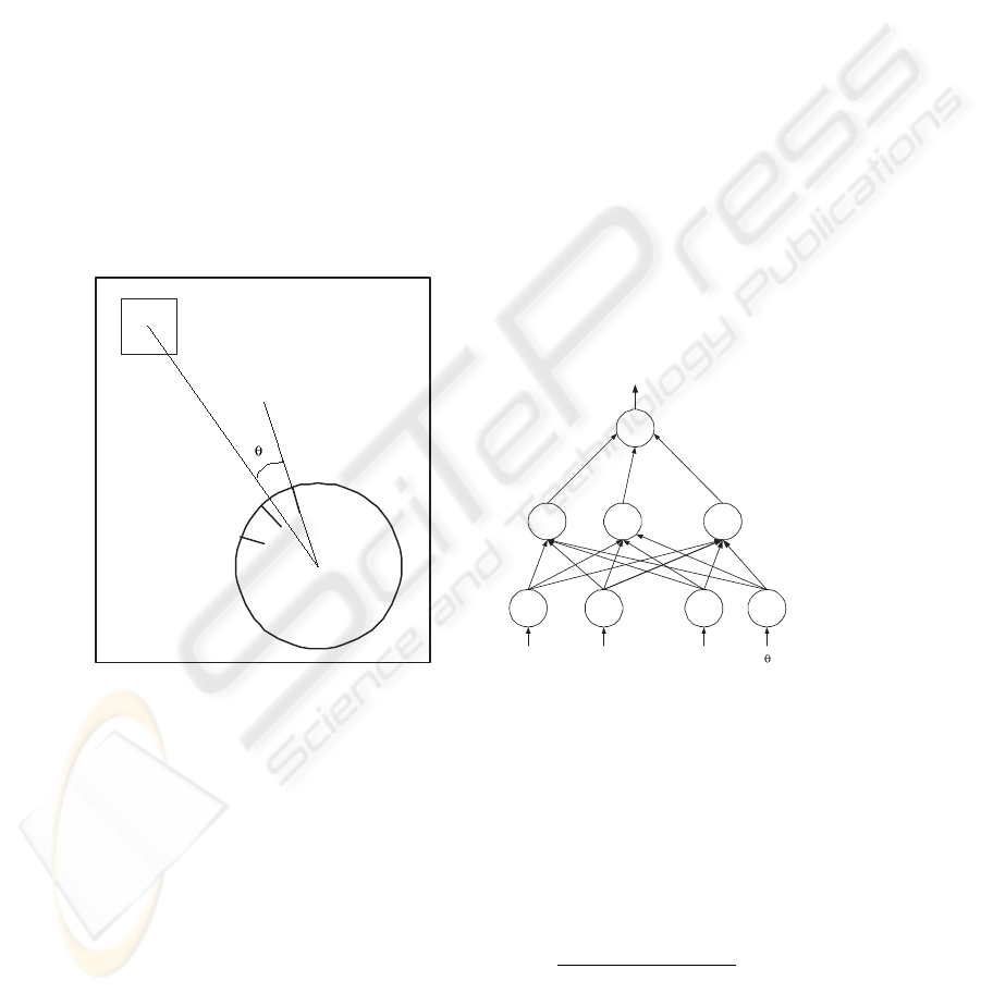
For each cell (i, j) ∈ G, where G is the grid in question, the input for the network

N is a vector of data that consists of two sonar readings s = (s

, s

) whose direction

is oriented by (i, j) and by the polar coordinates of the cell centre (i, j) related to the

robot, where θ

is the relative angle to the two sensors closest to the cells and d

is the

distance relative to the robot centre (see ﬁgure 1).

The output of the network is a probabilistic value that indicates the probability of

the cell being occupied (see ﬁgure 2).

s1

s2

s3

d

(i,j)

Robot

Fig.1. Sonar readings and robot angle and

distance to a cell(i,j)

. . .

s1

s2 d

Input Layer

Hidden Layer

Output Layer

Fig.2. Neural Network used for sensorial

reading interpretation

The neural network is used while the robot follows the obstacle edge.

Let M be the number of consecutive readings of sensors s

, s

, ..., s

, then the

occupancy probability of cell (i, j) can be seen as P rob(occ

, s

, ..., s

). If the

Bayes rule is applied to estimate the probability, the integration in time is obtained by:

P rob(occ

, s

, ..., s

) = 1 − (1 +

m=1

P rob(occ

)

1 − P rob(occ

)

−1

(1)

The neuronal interpretation can compensate eventual errors due to sonar signal re-

ﬂexion and the time integration over consecutive interpretations produce an acceptable

but limited sensorial information provided by the sensors.

2.2 Identiﬁcation of Obstacles Edges

From the local occupancy grid, the neural interpretation of the sensors is approximated

by a line that will be further used to build the set of partitions P .

A threshold ε is then established to deﬁne a limit to the cells (i, j) that will be

considered occupied P rob(occ

) > 1−ε. To calculate the straight line that deﬁned the

obstacles limits, a version of X

[7] is used.

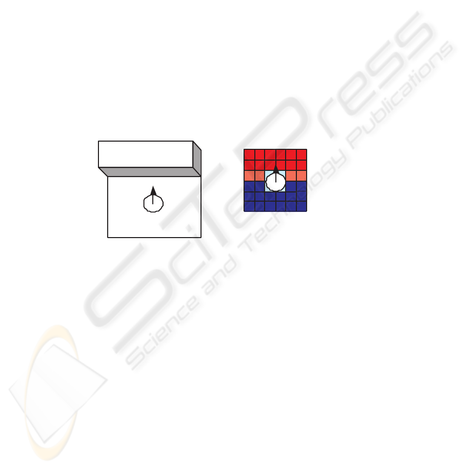
Figure 3 shows the step were the robot stops exploration to start mapping the obsta-

cle. The correspondent nxn occupancy grid to this local representation after the prob-

abilities achievement described before is shown by the different colors that represent

each cell in the grid. The red cells are those whose level of occupation is maximum, the

intermediate red represent a cell less occupied, while the light blue cells, were the robot

is located, are set to 0.5. The empty cells are colored with blue.

Local Grid Correspondent

Occupation

Fig.3. Occupancy grid representation for obstacle mapping

After the application of X

, each time the robot extracts a line from an obstacle,

it searches for a previous extracted line that can be aligned to it and whose orthogonal

distance between them is smaller than a threshold d.

The precision of the partitions depends on two factor: the grid local resolution and

the precision of the lines that approximate the obstacles.

2.3 Partition Updating

Every time the robot perceives an unknown obstacle it decides to increase the resolution

of the partitioning to model it.

From the initial identiﬁed corner to the last, the robot approaches the obstacle such

that: it aligns with one of its boundaries; it follows that boundary and starts using the

local grid and the method; as soon as the robot ﬁnds the straight line that approximates

this ﬁrst boundary, it stops utilising the local grid that is, the neural sensor interpretation,

computing the intersection between the current straight line and the previous one to

identify the corner previously visited; the robot moves until the end of the boundary

using the raw sensor readings only, rotates to align with the new boundary and repeats

the process until it reaches the ﬁrst corner met [5].

Once all corners of an obstacle have been memorized, it is possible to increase the

resolution of the partitioning to model the new obstacle: each new corner is connected

to the closest perpendicular edge of one of the existing partitions. This strategy always

creates rectangular partitions.

Two avoid redundancy, adjacent partitions that represent either obstacle or free

space, can be merged to produce a rectangular partition. After updating the partitioning

the robot stores the knowledge concerning physical transitions between new partitions.

2.4 Environment Exploration

Although we are aware that intelligent exploration can facilitate the task achievement

of building maps, in this phase of the project, we are not concerned with it and a simple

controller that directs the robot to the obstacles without crashing is applied.

2.5 Planning and Acting

The planner module is responsible for calculating the best way to ﬁnd a target partition

through the whole set of partitions. From the current set of partitions P , the planner

derives a topological graph. In this graph, the nodes correspond to the partitions and the

arcs are obtained from the long time memory. The correspondent node to partition α is

connected to the node corresponding to the adjacent partition β.

Leaving the node that corresponds to the current partition, the planner searches for

a graph with the minor path to achieve the target node. Once the path is determined, the

low level planner calculates the trajectory for the robot through the adjacents partitions.

All paths followed by the robot are lines parallels to x and y axis.

2.6 Low Level Control

A module relative to the low level controls the movement of the robot, dealing with

small map inconsistences and possible mobile obstacles. This module is also used to

make the robot follow the edges of the new obstacles to be modelled.

3 Map Merging

One of the solutions provided to deal with the exploration need that arises from the

sensors incapability of representing a global environment is by using multi-robot sys-

tems. In this representation, each individual robot that explores the environment applies

map building techniques to represent its perception of the world. However, individual

maps do not solve the problem before mentioned neither take advantage of the multi-

agent system. By using this cooperative navigation, one can obtain the individual maps

built by the robots and apply proper techniques to merge them into a single one that

results in global representation of the previously unknown environment. Furthermore,

it is expected that working in this way, one reduces the map building need of individual

exploration, although a merging technique, that does not represent a simple task, has to

be implemented.

In this work, although we have topological and geometric characteristics in our

resultant map, for merging purposes, only the topological information will be required,

leaving the geometric data available for future improvements that can become necessary

in the algorithms (the nodes could contain information about area size, distance between

nodes, etc.).

Robots that have explored overlapping regions of the environment should have topo-

logical maps that have common subgraphs with identical structure. Thus, solving a map

merging is the same as identifying a matching between two graphs [8].

If there is information about edges, i.e., path shapes and the orientations of the edges

and vertices, the location of the vertex can be estimated with respect to the robot’s frame

of work. One of the techniques that can be applied to solve this problem is part of the

class of algorithms called Iterative Closest Point (ICP) [9].

The algorithm proposed by [8], consists of basically creating hypotheses by locally

growing single-vertex matches. A hypothesis is a list of vertex and edge correspon-

dences between two maps; to ﬁnd them means, basically, to deﬁne all maximal common

connected subgraph matchings between those maps.

4 Results

4.1 Setup

The experiments were carried out on simulation. The tool used for modelling the en-

vironment and implement the algorithms was the Player/Gazebo simulator [10]. It is a

client/sever interface in which the server (Gazebo) works as a graphical interface and

provides the simulation data to each client (Player), connected to it. Each robot added

to the system requires a player associated to it, so that they can execute independent

algorithms.

The world modelled was speciﬁc for each task, as described later, with one or two

Pioneer2DX mobile robots working on it. The sensors used were 16 sonars and odom-

etry.

The experiments consisted on the robot(s) exploring the environment without much

concern about exploration details. As mentioned before, the map building algorithm

only stops performing exploration when it faces an obstacle. At this point, a model of

the object is deﬁned through the application of occupancy grid technique associated

with the neural networks weights.

Each occupancy grid has a 14x14 cells resolution, with each cell measuring 10x10cm

and the robot positioned in the middle of the grid (on the 4x4 central cells).

The neural network used to generate the occupancy grid was a feed-forward archi-

tecture trained with the backpropagation [11] algorithm with momentum term [12] to

minimise cross-entropy [11]. The ofﬂine training was executed in the NevProp toolkit

[13], whose resultant weights matrix was applied to the map building algorithm de-

scribed in section 2. The parameters of the network were:

– activation function = logistic

– initial neurons weight = ±0.001

– learning rate = 0.01

– maximum value of weight magnitude = 1.75

– momentum factor = 0.01

– decaying weigh factor = -0.001

The experiment lasted until the robot met the same initial corner it ﬁrst mapped.

4.2 Map Building

The performance of the algorithm to build cognitive maps based on the technique men-

tioned before are presented in this section.

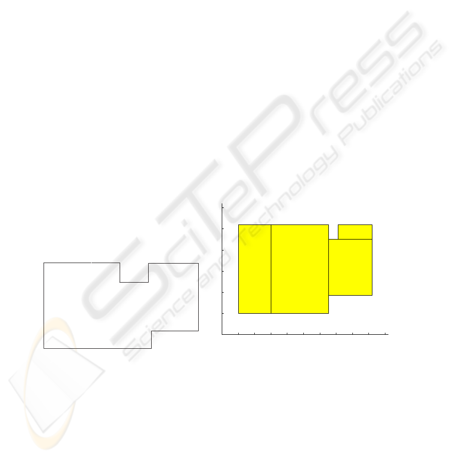
Figure 4 presents the world deﬁned for the task were only a single robot was applied.

The area represents the empty space and the edges correspond to the obstacles. Figure

5 shows the map resultant from the robot interaction. It can be noted that the acquired

model is a close representation of the real one and the small discrepancies that can be

veriﬁed on the middle top obstacle are caused mainly because of odometric error that

accumulates with time.

Fig.4. World model for the ﬁrst experiment

−1 0 1 2 3 4 5 6 7 8 9

−1

Fig.5. Map generated by a single robot working

in the environment

The second experiment, represented by ﬁgures 6 and 7 are the acquired models for

each of the two robots that are interacting with the world. They represent almost the

same graphic, though they have different perspectives. It was also perceived during the

experiments that the algorithm produces most of the time, even for the same robot with

the same initial condition, different partitions.

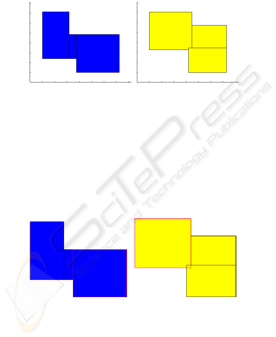
−1 0 1 2 3 4 5 6 7

−1

Fig.6. Map generated by robot 1

−1 0 1 2 3 4 5 6 7

−1

Fig.7. Map generated by robot 2

4.3 Map Merging Expected Results

If we apply the algorithm of map merging mentioned in section 3, the ﬁrst step to be

considered is the numeration of the corners of the graphics. Once each corner of each

map is identiﬁed, the hypothesis of possible combinations are established. For a 180

rotation carried on map 2 (Figure 9), the best hypothesis is:

a1 b1

c1 d1 e1

f1g1

h1i1j1

Fig.8. Map generated by robot 1

a2 b2

c2 d2

e2

f2g2

h2i2

Fig.9. Map generated by robot 2

a1 = f2

j1 = d2

h1 = c2

g1 = b2

f1 = a2

e1 = i2

d1 = h2

The red lines represented in ﬁgures 8 and 9 indicate the length of the vertices that

will be used to the establishment of relationships among the maps.

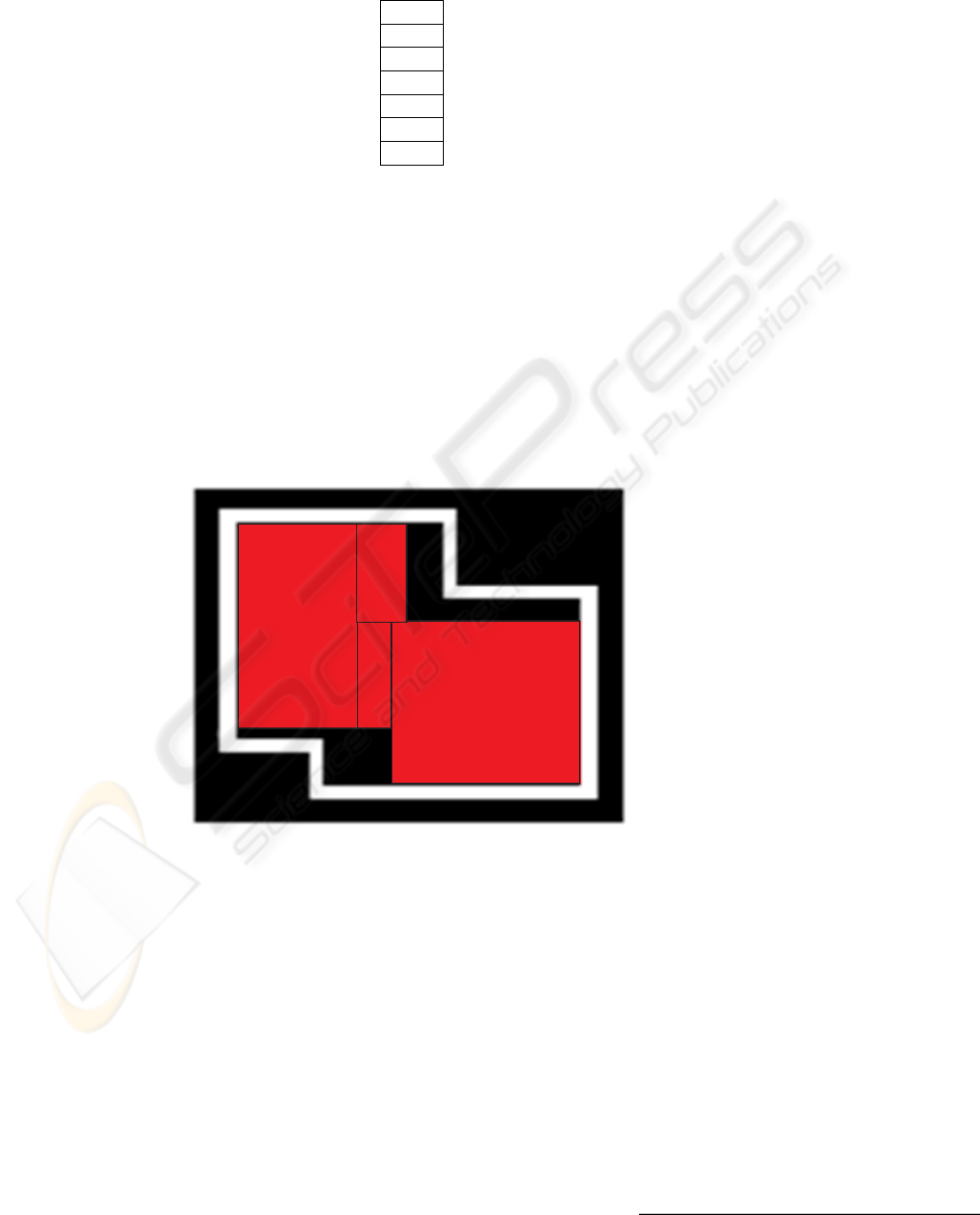
The resulting expected global map for the readings carried by robot 1 and 2 on the

same environment can be seen in ﬁgure 10. The red rectangles represent the global

map that is expected to be achieved by the application of the merging algorithm on

the previous individual maps. The black and white parts represent the real world map

used for simulation. It can be noted that, although we have proposed multi-agents to be

employed to decrease the need for exploration, at this point of the research, as no esti-

mation ﬁlter (such as Kalman) is used to correct the odometry errors, it is not possible

to run the robots on larger worlds, were they would have less overlapping regions and

the beneﬁts of map merging would be more clear.

Fig.10. Global expected map after merging

5 Conclusions and Future Work

The world models that result from the application of the map buildingtechnique achieved

a good trade-off between representation accuracy and learning efﬁciency. Although the

built maps did not represent the world precisely, the response is quite accurate if its

taken into account that only sonars and odometry were used to provide sensorial reading

and no ﬁlters are applied to estimate and correct the cumulative error drift that emerges

when the robot works in large environments. The variable size of the partitions allows

high resolution to be applied only when necessary (close to obstacles), what requires

less storage requirements.

References

1. Thrun, S.: Robotic mapping: A survey. (2002)

2. Thrun, S.: Learning maps for indoor mobile robot navigation. Artiﬁcial Intelligence 99

(1998) 21–71

3. Elfes, A.: Sonar-based real world mapping for navigation. IEEE Journal of Robotics and

Automation 3 (1997) 249–265

4. Wallner, F., Kaiser, M., Friedrich, H., Dillmann, R.: Integration of topological and geomet-

rical planning in a learning mobile robot. (1998)

5. Arleo, A., del R. Mill

an, J., Floreano, D.: Efﬁcient learning of variable-resolution cognitive

maps for autonomous indoor navigation. IEEE Transactions on Robotics and Automation 15

(1999) 991–1000

6. Moravec, H.P.: Sensor fusion in certainty grids for mobile robots. Artiﬁcial Intelligence 9

(1988) 61–74

7. H, P.W., A, T.S., T, V.W., P, F.B.: Numerical Recipes in C. Cambridge University Press

(1992)

8. Huang, W., Beevers, K.: Topological map merging. Proceedings of the 7th Intl. Symp. on

Distributed Autonomous Robotic Systems (2004)

9. Besl, P.J., McKay, N.D.: A method for registration of 3-d shapes. IEEE Trans. Pat. Anal.

and Mach. Intelligence 2 (1992) 239–256

10. Gerkey, B., Howard, A., Vaughan, R., Koenig, N., Howard, A.: Player/stage project (2004)

Dispon

ıvel em: <http://playerstage.sourceforge.net/>. Acesso em: Fevereiro 2005.

11. Bishop, C.M.: Neural Networks for Pattern Recognition. Oxford University Press, UK

(1995)

12. Rumelhart, D.E., Hinton, G.E., Williams, R.J.: Learning representation by back-propagation

errors. Nature 323 (1986) 533–536

13. Goodman, P.H.: NevProp3 User Manual, University of Nevada. (1996)