SVM Classification of Sparse Set of 1:1 Ventricular and
Supraventricular Tachycardia
Mario de-Prado-Cumplido
1
,
´
Angel Arenal-Ma
´
ız
2
, Mercedes Ortiz-Pat
´
on
2
and
Antonio Art
´
es-Rodr
´
ıguez
1
1
Department of Signal Theory and Communications, Universidad Carlos III de Madrid,
Avda. de la Universidad 30, 28911 Legan
´
es-Madrid, Spain
2
Laboratory of Cardiac Electrophysiology, Hospital General Universitario Gregorio Mara
˜
n
´
on,
C. Doctor Esquerdo 46, 28007 Madrid, Spain
Abstract. Inappropriate classification of Supraventricular Tachycardias with 1:1
atriovetricular conduction is a mayor issue in dual-chamber implantable cardio-
verter defribillators. In order to distinguish Supraventricular from Ventricular
Tachycardias a new methodology is proposed. The tachyarrhythmia episodes
ECGs are characterized into feature vectors, which are then classified using a
Support Vector Machine. The best features of the vectors are selected by means
of several Feature Selection methods. The performance of the algorithm over-
comes existing algorithms for implantable devices.
1 Introduction
Despite automatic implantable cardioverter-defibrillators (AICDs) show a very good
performance dealing with heart diseases, inappropriate therapies are still a mayor issue.
New generation of dual-chamber AICDs have the ability to take into account atrial-
ventricular relationships, and in particular, to detect the chamber which originates the
tachycardia. Nevertheless, the reduction of inaccurate detection of this new devices
have not been totally proved, specially for tachycardias with a stable 1:1 atrioventricular
relationship.
In this paper we tackle the problem of discriminating Supra Ventricular Tachycar-
dias (SVT) from Ventricular Tachycardias (VT) with 1:1 conduction; this property is
the main cause of the high complexity of the problem. Although the frequency of oc-
currence of this arrhythmias is low, inappropriate therapies (i.e., small specificity) cause
annoyance in the patient and may initiate a more compromising tachyarrhythmia. (See
for example [2], [1]). Usually data bases of pathological episodes are of reduce size,
which constitute and additional difficulty to bound the statistical accuracy of the re-
sults.
The electrocardiogram (ECG) of the tachyarrhythmia episodes is registered in the
AICDs as sequences of intervals between beats times. The difference between adjacent
intervals, known as Heart Rate Variability (HRV), has been of great interest for the re-
search community in the last decades, due to HRV signals gather information about the
complex processes that controlls the heart behavior [3]. We aim to implement SVT/VT
classification based in these HRV signals.
de-Prado-Cumplido M., Arenal-Maíz Á., Ortiz-Patón M. and Artés-Rodríguez A. (2005).
SVM Classification of Sparse Set of 1:1 Ventricular and Supraventricular Tachycardia.
In Proceedings of the 1st International Workshop on Biosignal Processing and Classification, pages 95-101
DOI: 10.5220/0001195600950101
Copyright
c
 SciTePress

The classification step is carried out with a classifier known as Support Vector Ma-
chine (SVM), which is the state-of-the-art technique for knowledge discovery and clas-
sification tasks, among others applications [5], [6], and is well founded in the Statis-
tical Learning Theory. The SVM classifiers have shown competitive results applied to
datasets with low ratio sample-size/number-of-dimensions, property very useful for our
problem. The characterization process of the HRV signals we have implemented is over-
informative, so Feature Selection (FS) methods must be applied in order to choose the
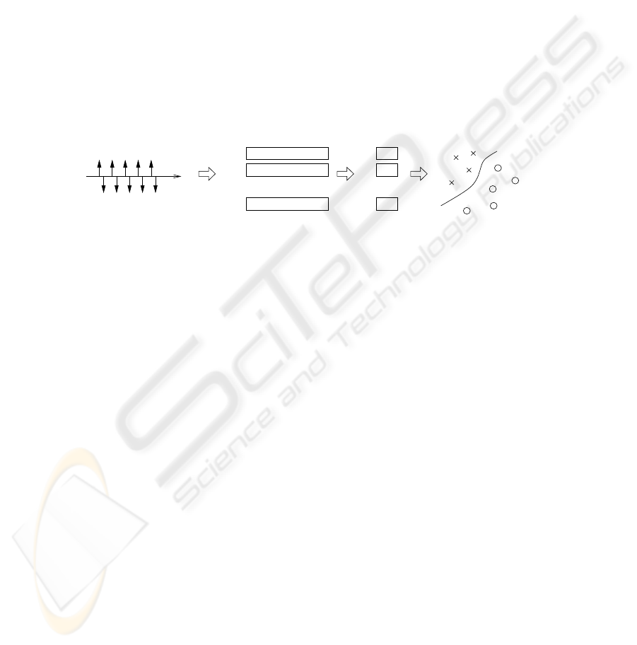
most informative variables. Our overall process for SVT-VT classification can be seen
in Figure 1.
This methodology was applied to 1:1 tachycardia episodes obtained from a Spanish
hospital, Hospital Gregorio Mara
˜
n
´
on (Madrid, Spain). We will show that the algorithm
we present increases the specificity percentages of present AICDs devices, while main-
taining 100% of sensitivity.
n
1
2
AA series
VV series
t
... ...
Feature
Selection
Characterization SVM Classification
n
Heart Rate Signals
1
2
Fig.1. General summary of the methodology. The heart rate intervals signals are coded into a set
of characterization vectors; the best features are fed into a SVM classifier
The paper is structured as follows: Section 2 explains the medical problem, the
signals used and its characterization vectors. Section 3 details the methodology imple-
mented, while the results are described in Section 4. Finally, the paper is closed with
some final remarks in Section 5.
2 Definition of the medical problem and the data
Ventricular Tachycardias (VT) and supraventricular ones require different therapies; in-
appropriate shocks for SVTs can induce a ventricular arrhythmia. The main criterion to
distinguish them is to identify the chamber responsible of the origin of the tachycardia.
This is specially problematic with stable atrioventricular relationship, i.e, when there is
a 1:1 conduction.
The episodes are registered in the AICDs (model 7276 Gem III AT; Medtronic Inc.)
as the sequence of interval times from beat to beat in each chamber. Assuming that a
i
contains the times of the beats in the atria, the atrial HRV is {aa
1
, ··· , aa
r
, ···} =
{a
2
− a
1
, ··· , a
r+1
− a
r
, ···}. In the same way, the ventricular HRV is
{vv
1
, ··· , vv
r
···} = {v
2
− v
1
, ··· , v
r+1
− v
r
, ···}, where v
i
are the instants for
ventricular beats. The series used in our study are based in those sequence of intervals:
s
1
(i) = {aa
r−24+i
− vv
r−24+i
} (1)
s
2
(i) = {aa
r−24+i
− vv
r−25+i
}
96

where i = {1, 24} and v
r
and a
r
are the last beats previous to the tachycardia detec-
tion instant according to the AICD criteria. We have focused only in this 24 intervals
{aa
r−23
, ··· , aa
r
} and {vv
r−24
, ··· , vv
r
} because it is the minimum time needed by
the AICDs to decide SVT or VT for the different episodes. The actual labelling has
been set inspecting the episodes stored in the AICDs. Classical algorithms for classi-
fying VTs are related with onset and stability of the variability; take into account that
s
1
(i) and s
2
(i) contains not only this information but indications about the chamber of
origin of the tachycardia.
Typical measurements of variability include mean and variance calculation, as well
as frequency domain or geometrical calculations or more complex ones as mutual infor-
mation (see [4] for explanation on these measures). We have chosen the mean and vari-
ance of the complete series s
1
and s
2
, the mean and variance of groups of 4 intervals,
and the mean and variance of these latter values. Consequently, for each tachycardia
episode a 32-dimension features vector is set.
3 Design of the classification method
This section describes the algorithms used in our classification scheme. Feature Selec-
tion algorithms have been applied to the SVT and VT vectors, characterized as describe
previously, in order to improve the error probability (in terms of sensitivity and speci-
ficity) and to discover the features that better describes the tachycardias. The episodes
are then classified with a SVM, obtaining both linear and nonlinear boundaries for the
decision regions.
3.1 Feature Selection
Feature Selection (FS) methods are used as a preprocessing step in classification prob-
lems, in which datasets are commonly composed of samples of two variables [7].
Consider a set of l tachyarrhythmias represented by the value of their n = 32
characteristics (constructed as explained in the previous section): (x
i
, y
i
), where i =
1, . . . , l, x
i
∈ R
n
, and the set labels y
i
∈ {−1, 1} denotes whether the arrhythmia is a
SVT (y
i
= −1) or a VT (y
i
= 1). In FS, the objective is to find a subset of components
of x that is optimal following a given criterion. The algorithms used in this article are
the well-known fisher score, Kolmogorov-Smirnoff test and Recursive Feature Elimi-
nation (RFE).
Fisher score method consists in computing the fraction F (i) =
(µ
+
− µ
−
)
2
(σ
+
)
2
+ (σ
−
)
2
,
where µ
+
and σ
+
are the means and variance of feature or dimension i (i ∈ 1, n)
for samples with label y
j
= +1; µ
−
and σ
−
are calculated for samples y
j
= −1.
Fisher FS is a linear method which maximizes the separation of the mean of the classes
while forcing minimum interclass variance. Kolmogorov-Smirnov test, a nonlinear FS
algorithm, ranks more favorably the features with mayor statistical relation with the
labels, through this equation: KS(i) =
√
n sup
n
ˆ
P (X ≤ f
i
) −
ˆ
P (X ≤ f
i
, y = 1)
o
,
where f
i
is the i-th feature and
ˆ
P the corresponding empirical distribution. Finally,
97

RFE runs for n iterations eliminating in each of them the feature that modifies the least
the probability error of the classifier. The two former FS methods are filter algorithms,
while the latter belongs to wrapper methods, because RFE takes into account the output
of the classifier to estimate the ranking of features.
Fisher criterion, Kolmogorov-Smirnov test and RFE has been applied to our data
set, and the more informative features has been used to train the classifier.
3.2 Support Vector Machine Classifiers
The nonlinear SVM classifier maps the input variable x
i
into a high dimensional (of-
ten infinite dimensional) feature space, and applies a maximum margin algorithm with
regularized complexity in this feature space. All the appearances of the mapping φ
are within dot products, which can be substituted by a kernel function. The nonlinear
SVM with kernel K(·, ·) = φ(·)φ(·) is equivalent to a regularization problem in the
reproducing kernel Hilbert space H
K
: minimize the functional,
1
2
kwk
2
+ C
l
X
i=1
ξ
i
(2)
subject to
y
i
(w
T
φ(x
i
) + b) ≥ 1 −ξ
i
∀i = 1, . . . , l
ξ
i
≥ 0 ∀i = 1, . . . , l
Once found the optimum w, the mappings of the SVMs for unseen samples x are
of the form
ˆy(x) = sign

w
T
φ(x) + b

(3)
where bias b can be used to generate a pseudo ROC curve and adjust the balance be-
tween errors of type ˆy
i
= 1|y
i
= −1 (miss error) and ˆy
i
= −1|y
i
= 1 (false alarm
error).
In this article we have used two kernels: the linear kernel (K (x
i
, x
j
) = x
T
i
x
j
) and
the well-known Gaussian Kernel, K (x
i
, x
j
) = exp

−γkx
i
− x
j
k
2

, where γ controls
the width of the Gaussian. The former presents a higher probability of error, but has
the advantage of being more interpretable, while gausian kernel has a more accurate
performance at the expense of simplicity in the solution. Simulations have been run
with both kernels.
The tunable parameters C and γ and the error probability (sensibility and speci-
ficity) of the SVM are estimated by a cross-validation approach. The SVM is trained
with all the episodes except one, and the result is evaluated for that sample. The proce-
dure is repeated for all the episodes, and the final figures are an average of all the steps;
this procedure is known as Leave-One-Out, and tends to generate slightly pessimistic
error probabilities.
98

4 SVT vs VT Classification Results
A set of 61 arrhythmias, 40 SVTs and 21 VTs, all of them showing a 1:1 conduction,
has been processed as explained in Section 2. In order to obtain confidence margins for
the results and assure their statistical validity, we have used a bootstrap resampling (see
[8]) of the episodes, with 15 resamples, so the specificity is expressed as the mean of
the estimator plus its standard deviation. Bootstrap errors are calculated by evaluating
repeatedly the estimator under study, that in our case are the SVM error probabilities.
The best performance, in terms of sensibility (
#ˆy=1|y=1
#y=1
) and specificity
(
#ˆy=−1|y=−1
#y=−1
), were obtained when the SVM was trained with the top 4 ranked vari-
ables according to the Kolmogorov-Smirnov test. RFE chose approximately the same
features, specially for the top rated ones. Fisher score selected other features, but the er-
ror probability of the SVM has been worst, due to the linear behavior of this FS method.
The meaning of the selected features are related with means and standard deviations of
series in eq. (1), as explained in Table 1.
Table 1. Four best features according to Kolmogorov-Smirnov test and their meaning
No. of feature Meaning
f
6
mean of the full inter-chamber HRV, s
2
f
10
mean of {s
2
(13), s
2
(16)}
f
7
mean of {s
2
(1), s
2
(4)}
f
16
standard deviation of {s
2
(5), s
2
(8)}
−2 −1 0 1
−2
−1.5
−1
−0.5
0
0.5
1
f
6
f
10
−2 −1 0 1
−2
−1.5
−1
−0.5
0
0.5
1
f
6
f
10
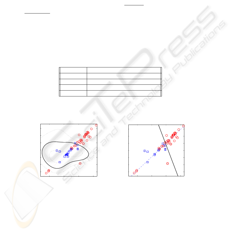
(a) (b)
Fig.2. Example of a) non-linear and b) linear classifiers. Squares and circles represent VTs and
SVTs, respectively. The continuous curves is the boundary between the two types of tachycardias
Two types of SVM classifiers has been proved, a nonlinear gaussian and a linear
one. In Figure 2 an example of a classification with only 2 variables, f
6
and f
10
, is
shown. Note that the boundary between both classes (squares for SVT and circles for
99

VT) is clearly a non-linear curve. In this case, 4 SVTs have been considered as VTs. The
dashed line represent the direction of maximum variance of the data set when only those
variables are taken into account. It would be easy to implement an algorithm that with
just 2 thresholds: check if the episode is in the upper right or bottom left areas of the
figure, and decide then that it is a SVT case, or, otherwise, decide a VT. For the linear
SVM drawn in Figure 2 b) a simple classification rule can be derived: if (f
6
> 200)
AND (f
10
> 195) decide VT (the values in the figure are normalized).
Table 2 shows the performance of the SVMs, depending on the number of vari-
ables. Classification with more than 4 variables performs worse in term of sensibility
and specificity. As mentioned before, specificity values include their bootstrap standard
error. Sensibility, on the contrary, has been forced to be 100%, at the expense of a lower
specificity; this has been done adjusting conveniently the bias parameter b of the SVM.
For comparison, in [1], a study with data from AICDs showed a 60% of specificty
in VT/SVT detection; the set of tachycardies in this case includes both 1:1 conduction
SVTs and normal SVTs. In [2], 160 SVTs episodes were used, only 16 of them showing
1:1 conduction. Although the algorithm used in [2] shows an 89% specificity, all 16 1:1
SVTs were misclassified. Consequently, the proposed methodology clearly overcomes
existing algorithms for AICDs.
Table 2. Results for both linear and non-linear SVMs, for the most informative features; we also
include the parameters of the best classifier
Non-linear Classifier Linear Classifier
#features Sensibility Specificity Params Sensibility Specificity Params
2 100 89.95 ± 3.90 C : 100, γ : 2 100 80.80 ± 6.97 C : 100
3 100 88.60 ± 5.71 C : 100, γ : 3 100 79.91 ± 6.73 C : 10
4 100 85.57 ± 4.88 C : 100, γ : 4 100 77.28 ± 8.17 C : 10
5 Conclusions and Further Work
In this paper we present a methodology for discriminate 1:1 ventricular tachycardias
from supraventricular ones, based on real signals from dual-chambers AICDs. This
pathology constitute a mayor issue due to existing algorithms do not perform with a
satisfactory level of specificity. Additionally, the occurrence frequency of this tach-
yarrhythmias is low, and the size of our data base is consequently small. The presented
methodology has obtained results that improve the specificity of existing AICDs algo-
rithms.
Our methodology could be used to explore other measurements on the HRV, just
creating new feature vectors without modifying the rest of the algorithms; new mea-
surements coul be based, for example, in mutual information or morphological criteria.
In order to implement SVM classifier into the AICD devices it would be necessary to
study and reduce its computational burden.
100

References
1. Theuns, D.A., Klootwijk, A., Goedhart, D., Jordaens, L.: Prevention of Inappropriate Therapy
in Implantable Cardioverter-Defibrillators Journal of the American College of Cardiology,
Vol.44, No.12, (2004)
2. Kouakam, C., Kacet, S., Hazard J.R. et al.: Performance of a Dual-chamber Implantable De-
fibrillator Algorithm for Discrimination of Ventricular from Supraventricular Tachycardia.
Europace, 6, (2004), 32-42
3. Malik, M., Camm, J., (eds.): Heart Rate Variability. Futura, Nueva York (1995)
4. ESC/NASPE Task Force: Heart Rate Variability: Standards of Measurement, Physiological
Interpretation and Clinical Use. European Heart Journal, Vol.17, (1996), 354-381
5. Sch
¨
olkopf, B., Smola, A.: Learning with Kernels. MIT Press, Cambridge, MA (2002)
6. Rojo-
´
Alvarez, J.L., Arenal-Ma
´
ız, A., Art
´
es-Rodr
´
ıguez, A.: Discriminating between Supraven-
tricular and Ventricular Tachycardias from EGM Onset Analysis. IEEE Engineering in Medi-
cine and Biology Magazine, Vol.21, No.1, (2002)
7. Guyon, I., Weston, J., Barnhill, S., Vapnik, V.: Gene Selection for Cancer Classification Using
Support Vector Machines. Machine Learning, Vol.46, No.1-3, (2002)
8. Efron, B., Tibshirani, R.: An Introduction to the Bootstrap. Chapman & Hall (1993)
101