
HRV Computation as Embedded Software
George Manis
University of Ioannina
Dept. of Computer Science
P.O. Box 1186, Ioannina, 45110, Greece
Abstract. The heart rate signal contains useful information about the condition
of the human heart which cannot be extracted without the use of an information
processing system. Various techniques for the analysis of the heart rate variability
(HRV) have been proposed, derived from diverse scientific fields. In this paper we
examine theoretically and experimentally the most commonly used algorithms
as well as some other interesting approaches for the computation of heart rate
variability from the point of view of the embedded software development. The
selected algorithms are compared for their efficiency, the complexity, the size of
the object code, the memory requirements, the power consumption, the real time
response and the simplicity of their interfaces. Figures giving a rough image of
the capability of each algorithm to classify the subjects into two distinct groups
presenting high and low heart rate variability are also presented, using data ac-
quired from young and elderly subjects.
1
1 Introduction
Heart rate variability is a research topic which constitutes the interest of many re-
searchers causing the number of publications in the field to increase day by day and
different algorithms and application methods to be examined. Heart rate variability
refers to the beat-to-beat alterations in heart rate. Various analysis methods have been
proposed which can be categorized as statistical, geometrical, frequency and time de-
composition analysis methods as well as non-linear ones. Guidelines for standards and
measurement are summarized in [1]. A summary of measures and models is presented
in [2]. A review article examining the physiological origins and mechanisms of heart
rate can be found in [3].
Embedded systems are small computing components designed to constitute part of
other, larger systems, e.g. electrical appliances, medical devices, etc. They consist of
software modules usually running on low-cost processors dedicated to perform specific
tasks; for example the task which controls the anti-block system of a car can be as-
signed to a specific processor. Algorithms developed for such systems have different
philosophy than those designed for general purpose computing systems, where power-
ful processors and almost unlimited resources have been assumed. The design of light-
weight embedded software algorithms for the computation of HRV is an interesting
1
This research was funded by the European Commission and the Greek Ministry of Education
through EPEAEK II
Manis G. (2005).
HRV Computation as Embedded Software.
In Proceedings of the 1st International Workshop on Biosignal Processing and Classification, pages 150-157
DOI: 10.5220/0001195401500157
Copyright
c
SciTePress

problem and to the best of the author’s knowledge no previous work has been done
towards this direction.
In this paper we study the most widely used algorithms for HRV analysis. As a
basis the guidelines suggested in [1] are used. All methods presented there for the com-
putation of HRV are examined. Some alternative approaches are also investigated. The
intention is not to construct an embedded system which calculates the variability of the
heart rate signal but study algorithms for this purpose. Thus, we work only in software
level and take into consideration the effect of the software level in the system hardware.
2 Requirements and Design Choices
The design philosophy of an embedded system is very different from that of a con-
ventional software application. In the latter the application developers take only very
primitive decisions about the hardware or the operating system; they select the underly-
ing architecture based on commercial criteria (number of available machines, possible
customers, etc.).
Things are very different when designing an embedded system. Money still makes
the world go round, but the target now is a very specific task for a very specific architec-
ture. Decisions should be made in both hardware and software levels, the one affecting
the other in a remarkably high degree. We isolate the factors that affect those decisions
and are related to our problem.
It is not a new or surprising request that every information processing system has
to produce accurate and reliable results. The accuracy of the computation is connected
with the capability of the algorithm to classify the subjects correctly. It should be noted
that the problem of selecting the best algorithm with unbiased classification is still open,
lot of research has been done and is still to be done. In this paper we present the results
of our experiments to give an indication of the ability of each method to classify the
subjects. We used three different sets of data but only one of these sets is presented here
since all results were similar.
An important factor which is of special interest and should be kept as low as possible
is the financial cost. Suppose an embedded architecture which is part of a widely used
electrical appliance. A small reduction in the cost may result into a huge amount of
money if multiplied with the number of appliances produced. The cost of the hardware
is mainly affected by the selection of the processor, and the memory capacity and speed.
The cost of the processor as well as the memory requirements depend on the com-
plexity of the algorithm, the size of the code, the necessary space for storing data and the
required system performance. We are interested in what we can do from the algorithmic
point of view in order to reduce these requirements as much as possible. Thus, we re-
design the algorithms and implement them in ANSI C. We use techniques like integer
arithmetic, shifting instead of divisions where possible, loop unrolling, replacement of
library function calls etc. and investigate all known techniques for code optimization.
We evaluate the produced algorithms for accuracy again, for efficiency, for the size of
the code and the memory requirements. The results are used for comparative study.
In order to calculate the above characteristics for each algorithm we use the JouleTrack
151

tool [4]. Experiments were performed for StrongARM SA-1100 processor for operating
frequency of 206MHz.
Another interesting issue in the embedded system design is the ability to produce
results in real time. We break this requirement into two smaller: (i) the time interval
between two successive sets of input data should be enough so that all necessary calcu-
lations are completed and (ii) the system should produce output in a constant rate and
for every set of input data. The second requirement is not always possible, necessary or
it can be very expensive.
In a HRV system the actual input is in general the ECG signal, from which the se-
quence of beats are constructed by proper algorithms for detection of individual heart-
beats. The rate of the heartbeats is approximately, one per second. Thus, necessary
calculations for each beat should be completed in one second, plenty of time for both
simple and complex algorithms. When for coherence and redundancy of results the
HRV index is computed with more than one algorithm in parallel, the one second time
interval may not be enough. In this case a more powerful processor and/or faster mem-
ory units might be necessary. The ability to produce results for every input beat instead
of only producing the final result at the end is desirable but not necessary. The physi-
cian needs only the final value of the index after all computations have been completed.
However, the capability of the algorithm to produce intermediate results is an interest-
ing feature. As an example consider the case of 24 hours recordings, where an early
approximation of the final result might be useful.
The growing importance of power consumption minimization affects drastically the
design of the embedded systems, since they are often part of mobile devices which
obtain energy through their batteries. The autonomy of these devices as well as the life
of the battery depend on the power consumption. Power consumption is mainly affected
by the selection of the processor and the memory system.
In order to have an estimation for the energy requirements we calculate the power
consumption for each algorithm. Each machine code instruction consumes a different
amount of power: indexed access to memory is more expensive than the direct one, mul-
tiplications are mode expensive than additions etc. We calculate the power consumption
of each algorithm using again the JouleTrack tool [4].
Another factor that affects the financial cost and the power consumption is the inter-
face of the software with the rest of the embedded system. The device that the physician
will use must provide the maximum information, however, sometimes it is possible to
simplify the application interface without affecting significantly the functionality, for
example a numerical display can sometimes substitute a graphical screen. The commu-
nication of an embedded software with the rest of the system is usually done through
specific hardware. Generally this is not expensive, however it should be kept to mini-
mal. In the HRV computation problem some algorithms produce only a single number
as an output while some other require a high definition graphical interface.
Finally, embedded systems are of low weight and small size. Mobile telephones are
typical examples where size and weight seems to be a challenge and affect drastically
the commercial value of the product. Small program size, low memory requirements,
low power consumption and simple application interface result into smaller and lighter
chips and batteries.
152

Day by day, the cost of the hardware is significantly reduced, processors are becom-
ing more and more powerful and memory capacities larger, while batteries are getting
smaller and smaller and much lighter. However, the need for efficient, lightweight, cost-
effective algorithms producing accurate and reliable results remains and will always be
interesting. Especially in problems like the HRV analysis, which finds application in
the development of wearable devices as well, the cost, the size and weight will always
be a challenge.
3 Methods
In [1] the most common methods for HRV analysis are presented. Examined here are the
standard deviation of RR intervals (SDNN), the standard deviation of the average RR
interval calculated in over short (usually 5 min) periods (SDANN), the square root of
the mean squared differences of successive RR intervals (RMSSD), the number succes-
sive RR intervals greater than x (usually 50ms) divided by the total number of intervals
(pNNx), the standard deviation of differences between adjacent intervals (SDSD), the
total number of all RR intervals divided by the height of the histogram of all NN inter-
vals (TI), the baseline width of the minimum square difference triangular interpolation
of the highest peak of the histogram of the intervals (TINN) and the power spectrum
density (PSD). We also examine the local linear prediction (LLP) and least squared ap-
proximation (LSA) which calculate the average prediction and approximation errors of
the timeseries [5] and the local fast approximation (LFA) which approximates the signal
with less accuracy but faster than LSA. Discrete Wavelet Transform (DWT) analyzes
the signal using wavelets and calculates the standard deviation in every scale of analysis
[2].
4 Implementation Issues
Several techniques for reducing the requirements of the embedded software develop-
ment were used in implementation level. The most interesting ones will be discussed in
this section trying to show how important the implementation level is and how much it
affects the system performance and the design choices at the hardware level.
We used integer arithmetic instead of a floating point one. Arithmetic operations
are much less expensive when operands are integer numbers. The size of an integer
in a typical processor is equal to the size of a word, usually much longer but never
smaller than two bytes even in low-performance cost-effective processors. An accuracy
of at least 2
16
levels for representing data has been proved more than acceptable for our
problem and does not affect the final results.
Next, we eliminated expensive operations and/or library calls. Library calls are usu-
ally expensive parts of computation, since most of the times they perform complicated
operations. Moreover, the calling mechanism increases the total execution time, the
memory requirements, the size of the object code and the power consumption. Although
this overhead is not always significant, it should not be ignored. We eliminated function
calls by modifying the algorithms where possible, or by replacing the call with other
operations more lightweight and faster.
153
Heuristic code optimization was also done depended on the the special charac-
teristics of each algorithms. Techniques like loop unrolling, reduction of the number
of memory accesses, or code size minimization can be characterized as heuristic ap-
proaches. We used the trial and error approach in the programming language level and
studied the effects in the assembly level. Some optimizations led to very good results.
5 Experimental Results
In this section we will present our experimental results. We will present graphs giving
indications about the capability of each method to classify subjects and tables with the
comparative experimental results for each algorithm including complexity, object code
size, memory and energy requirements and execution time.
Table 1. Comparative experimental for various HRV measures
SDNN SDANN RMSSD SDNNi SDSD pNN50 TI TINN
Obj. code before linking (KB) 1 1 0.9 1.1 1.3 1 0.9 0.7
Obj. code after linking (KB) 27 27 27 27 27 25 19 19
Obj. code linked & optim. (KB) 18 18 18 18 18 18 19 19
Memory requirements O(n) O(n/k) O(1) O(k) O(k+n/k) O(1) O(h) O(h)
Complexity O(n) O(n) O(n) O(n) O(n) O(n) O(n) O(n)
Average complexity O(n) O(n) O(n) O(n) O(n) O(n) O(n) O(n)
Exec. time before optim. (µs) 33381 8823 25541 33834 48269 17481 7738 7767
Exec. time after optim. (µs) 33381 2597 2319 3246 3154 2756 7738 7767
Power cons. before optim.(µJ) 11887 3142 9095 12048 17189 6225 2756 2775
Power cons. after optim.(µJ) 11887 925 826 1156 1123 981 2756 2775
Interface scalar scalar scalar scalar scalar scalar scalar scalar
Real time response no yes yes yes no yes yes yes
As mentioned in a previous section, the selection of the algorithm that categorizes
the subjects in an unbiased way is still open and is out of the scope of this paper. We
just present the results of our experiments to give a rough image of the classification
capabilities of each algorithm.
We used three different sets of data and the results were similar. The first set con-
sisted by 24 hours long signals from subjects with unremarkable medical histories and
normal physical examinations and subjects with angiographically confirmed coronary
disease. Recordings were acquired using a Holter device. The second set consisted again
of control and patient subjects with coronary artery disease. Each recording was ap-
proximately 2 hours long and acquired using a digital electrocardiograph in a hospital.
The experiments presented here used a third data set described in [6]. Five young (21 -
34 years old) and five elderly (68 - 81 years old) rigorously-screened healthy subjects
underwent 120 minutes of continuous supine resting while continuous electrocardio-
graphic (ECG) signals were collected. All subjects provided written informed consent
154
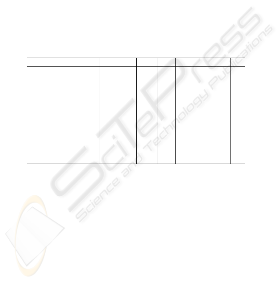
SDNN SDANN RMSSD SDNNi
SDSD pNN50 TI TINN
Fig.1. Categorization results for SDNN, SDANN, RMSSD, SDNNi, SDSD, pNN50, TI and
TINN. Circles (“o”) are for younger subjects and crosses (“+”) for elderly ones
and underwent a screening history, physical examination, routine blood count and bio-
chemical analysis, electrocardiogram, and exercise tolerance test. Only healthy, non-
smoking subjects with normal exercise tolerance test, no medical problems and taking
no medication were admitted to the study. All subjects remained in a resting state in si-
nus rhythm while watching a movie to help maintain wakefulness. The continuous ECG
was digitized at 250 Hz. Each heartbeat was annotated using an automated arrhythmia
detection algorithm, and each beat annotation was verified by visual inspection. The RR
interval time series for each subject was then computed. Figures 1, 2 and 3 present the
classification of subjects for all investigated algorithms.
Table 2. Comparative experimental for various HRV measures
LLP LSA LFA PSD DWT
Object code before linking (KB) 0.9 1.1 1.6 2.2 1.4
Object code after linking (KB) 25 27 26 28 27
Obj. code linked & optimized (KB) 18 19 19
Memory requirements O(k) O(k) O(k) O(n) O(n)
Complexity O(n
2
) O(n) O(n) O(nlog
2
n) O(n)
Average complexity O(nk) O(n) O(n) O(nlog
2
n) O(n))
Exec. time before optimiz.(µs) 65014 132981 50384 489748 477908
Exec. time after optimiz.(µs) 2994 5292 3575
Power consumpt. before optim. (µJ) 23151 47355 17942 174399 170183
Power consumpt. after optim.(µJ)
1066 1885 1273
Interface scalar scalar scalar vector vector
Real time response yes yes yes no no
155
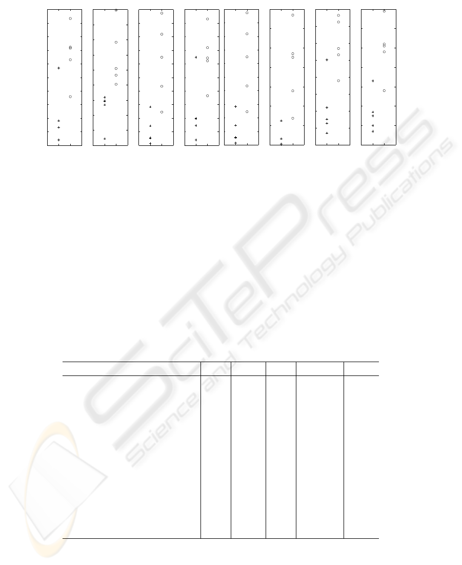
1 2 3 4 5 6 7 8
Categorization with Wavelet Decomposition
Scales of Analysis
Mean Length of Detail Coefficients
Fig.2. Left: Categorization results for Haar Wavelets Decomposition, dotted thin lines are for
elderly subjects and solid lines for younger ones. Right: Power Spectrum Density of a normal
subject (up) and a subject than presents decreased heart rate variability (down), the power in the
case of the elderly subject exhibits a continuous broadband spectrum
In the following, the experimental results presented in tables 1-2 will be discussed,
taking into consideration the size of the object code, the memory requirements, the
complexity, the execution time, the power consumption, the interface and the ability to
response in real time. Experiments were performed for StrongARM SA-1100 processor
for operating frequency of 206MHz using the JouleTrack tool[4].
The size of the object code is investigated before and after linking as well as after
the optimization. The size of the code before linking is interesting in the case in which
more than one HRV indices are implemented in embedded software. The optimized
code results from the application of the optimization techniques presented in a previ-
ous section. The differences appearing in tables 1-2 vary from 0.9KB to 2.2KB before
linking and from 18KB to 19KB after linking and optimization.
The complexity of the algorithms is O(n) in most of the cases, where n is the size
of the signal. An exception to the rule is the LLP algorithm which presents a relatively
high complexity O(n
2
). However the average complexity is only O(nk), where k is
the size of the sliding window and can be reduced to O(n) when the calculation of the
predicted value uses the value of the previously predicted point. The P SD calculation
present a complexity of O(nlogn).
The memory requirements have been computed in a similar way. The algorithms
SDN N, P SD and DW T need to store the whole signal in an array, thus the spacial
complexity is O(n). The calculation of the indices SDNNi, LLP , LSA, LF A need
to store only a vector with size k, equal to the size of the sliding window. The SDANN
metric requires O(n/k), since we need to store one value for each sliding window. The
same with SDSD, or more precisely O(k +
n
k
), since we also have to keep a vector
with the sliding window. TI and T INN use a vector of length h to store the histogram,
156

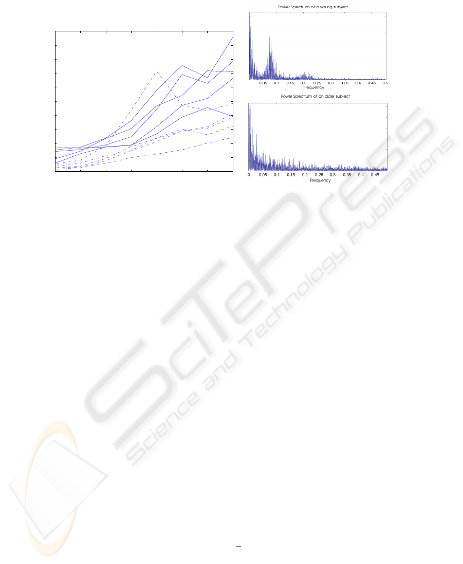
LLP
LSA LFA
Fig.3. Categorization results for LLP, LSA and LFA. Circles (“o”) are for younger subjects and
crosses (“+”) for elderly ones
where h is the size of the vector that stores the histogram. The memory required for the
calculation of the RMSSD and pNN x indices is constant and independent from the
size of the input or the parameters of the algorithm.
Experimental results for the execution time and the power consumption are also
presented before and after optimizations. The size of the input is 8192 samples and the
same input has been used for all algorithms. The differences for both execution times
and power consumption presented in tables 1-2 are sometimes remarkable. As long as
the interface of the system is concerned, all algorithms return a single value as a result
except the time and frequency analysis methods as shown in table 2, which produce a
vector of values. For these algorithms a graphical interface would also be useful. Apart
from the SDNN , P SD and DW T which require that the whole signal is available
before the first output is produced, all other algorithms can be considered as real time.
References
1. European Society of Cardiology: Heart rate variability, standards of measurement, physiolog-
ical interpretation and clinical use. European Heart Journal 17 (1996) 354–381
2. Teich, M., Lowen, S., Vibe-Rheymer, K., Heneghan, C.: Heart rate variability: Measures and
models. In: Nonlinear Biomedical Signal Processing Vol. II, Dynamic Analysis and Mod-
elling, New York (2001) 159–213
3. Berntson, G., Bigger, J., Eckberg, D., Grossman, P., Kaufmann, P., Malik, M., Nagaraja, H.,
Porges, S., Saul, J., van der Molen, P.S.M.: Heart rate variability: Origins, methods, and
interpretive caveats. Psychophysiology 34 (1997) 623–648
4. Sinha, A., Chandrakasan, A.: Jouletrack - a web based tool for software energy profiling. In:
Design Automation Conference. (2001) 220–225
5. Manis, G., Alexandridi, A., Nikolopoulos, S.: Diagnosis of cardiac pathology through predic-
tion and approximation methods. In: Seventh International Symposium on Signal Processing
and its Applications, Paris, France (2003)
6. Iyengar, N., Peng, C.K., Morin, R., Goldberger, A., Lipsitz, L.: Age-related alterations in the
fractal scaling of cardiac interbeat interval dynamics. Am J Physiol 271 (1996) 1078–1084
157
