
Foot Pathologies Classification From Pressure
Distribution Over The Foot Plant
⋆
Jos
´
e Garc
´
ıa-Hern
´
andez
1
, Roberto Paredes
1
, David Garrido
2
and Carlos Soler
2
1
Instituto Tecnol
´
ogico de Inform
´
atica
2
Instituto de Biomec
´
anica de Valencia
Universidad Polit
´
ecnica de Valencia
Camino de Vera s/n, 46071 Valencia (Spain)
Abstract. Nowadays, approximately 35% of the population suffers problems in
the feet. In many cases, some foot pathologies are treated by means of especial
insoles. These insoles require customisation for the success of their treatment.
However, there is a great lack of knowledge in this sector. As an initial step it
is essential to develop a new objective tool capable to classify among the dif-
ferent foot pathologies. In this paper we present a system to classify different
foot pathologies which uses the Nearest Neighbor (NN) classification rule based
on weighted metrics and prototypes selection. The system uses as input data the
pressure distribution over the foot plant.
1 Introduction
In the developed countries, approximately 35% of the population suffers problems in the
feet enough serious to need medical attention. The illnesses of the feet are recognised
as a great social problem in most of these countries, being most of the people affected
women. A high percentage of the population of the European Union over 40 years old
has some type of problem in their feet (above 90% in Spain, United Kingdom, Germany
or Holland).
In many cases, some foot pathologies are treated by means of especial insoles whose
principal aim is to protect the feet against external aggressions (overpressures, shear
forces, etc.) and to maintain the articulations in a suitable anatomical position. These
insoles require customisation for the success of their treatment. However, there is a great
lack of knowledge in this sector. On the one hand, there is not information regarding
the best orthetic solution depending on the pathology. On the other hand, in the health
area the final adaptation of the insole to the patient highly depends on the specialist
experience and on the capability of the patient to transmit the problems to the orthotics
use. This lack of knowledge, together with a low technology in the design process,
causes that the orthotics customisation process is performed at present without objective
criteria and in a traditional way which implies a process with low efficiency.
⋆
Work supported by the “Agencia Valenciana de Ciencia y Tecnolog
´
ıa (AVCiT)” under grant
GRUPOS03/031 and the Spanish Project DPI2004-08279-C02-02
Gar
´
cıa-Hernández J., Paredes R., Garrido D. and Soler C. (2005).
Foot Pathologies Classification From Pressure Distribution Over The Foot Plant.
In Proceedings of the 1st International Workshop on Biosignal Processing and Classification, pages 87-94
DOI: 10.5220/0001195200870094
Copyright
c
SciTePress

Therefore, as an initial step and taking into account the information presented above,
it is essential to develop a new objective tool capable to classify among the different
foot pathologies, disorders or problems in order to optimise and focus the strategies of
design to improve treatments and footwear functionality.
In this paper we present a system to classify different foot pathologies from pressure
distribution over the foot plant during walking. For this purpose, we compare the k-
Nearest Neighbor (kNN) classification rule using the well known Euclidean Distance
with the 1-NN classification rule improved by the Learning Prototypes and Distance
(LPD) method [1, 2]. While at section 2 we present the LPD method, at section 3 is
shown the database used in the experiments presented at section 4.
2 Methodology
The Nearest neighbor (NN) classification rule has successfully been used in many pat-
tern recognition applications. The good behaviour of this rule with unbounded number
of prototypes is well known. However, in many practical classification problems only a
small number of prototypes is usually available.
The NN performance can be improved by using appropriately trained distance mea-
sures of metrics. Improvements can be particularly significant for small prototype sets.
Trained metrics can be global (the same for all the prototypes [3–5], class-dependent
(shared by all the prototypes of the same class) [6–8] and/or locally-dependent (the
distance measure depends on the particular position of the prototypes) in the feature
space [9–12].
More concretely, in this work we have used (comparing with the well known Euclid-
ean Distance) the approach called Learning Prototypes and distances (LPD), proposed
in [1,2]. It stars with an initial selection of a small number of randomly selected proto-
types from the training set. Then it iteratively adjusts both the position (features) of the
prototypes themselves and the corresponding local-metric weights, so that the resulting
combination of prototypes and metric minimises a suitable estimation of the probabil-
ity of classification error. The adjustment rules are derived by solving the minimisation
problem through gradient descent.
2.1 Approach
Let T = {x
1
, . . . , x
N
} be a training set; i.e., a collection of training vectors or class-
labelled points x
i
∈ E, 1 ≤ i ≤ N in a suitable representation space. In our case, each
training vector (prototype) x
i
represents each subject. The components of this vector
are the pressure values of the subject’s plant foot acquired from a specific sensor. Being
M the number of available plant foot sensors, the training vector x
i
∈ R
M
, that is the
representation space E = R
M
. Each prototype belongs to a particular class, among C
different classes, being each class a different foot pathology.
The goal of the LPD algorithm is to use T to obtain a reduced set of prototypes,
P = {y
1
, . . . , y
n
} ⊂ E, n ≪ N, and a suitable weighted distance d : E × P → R
associated to P , which optimise the Nearest Neighbor (NN) classification performance.
Initially P is a subset of T randomly selected.
88

The weighted distance from an arbritrary vector x ∈ E to a prototype y
i
∈ P is
defined as:
d
W
(x, y
i
) =
v
u
u
t
M
X
j=1
w
2
ij
(x
j
− y
ij
)
2
(1)
where w
ij
is a weight associated with the feature j of the prototype y
i
. That is, in our
problem, w
ij
is the weight associated with the plant foot sensor j. These weights can
be represented as an N × M weight matrix W = {w
ij
, 1≤i ≤ N, 1≤j ≤ M }. In what
follows, whenever the weight matrix W can be understood from the context, d
W
(x, y
i
)
will be simply denoted as d(x, y
i
).
Note that this definition assigns separate weights to the different dimensions or fea-
tures of the representation space. Note also that it is asymmetric and local in that it
depends on the particular position of each y
i
.
Learning the Prototypes and their Weights In order to find both a matrix W and a
suitable reduced set of prototypes P that results in a low error rate of the NN classifier,
we propose minimise a criterion index which is an approximation to the NN classifica-
tion error of T using P and d(·, ·). This NN error estimate can be written as:
J(P, W ) =
1
n
X
x∈T
step
d(x, y
=
x
)
d(x, y
6=
x
)
!
(2)
where the step function is defined as
step(z) =
(
0 if z ≤ 1
1 if z > 1
and y
=
x
, y
6=
x
∈ P are, respectively, the same-class and different-class NNs of x. Note
that each term of the above sum (2) involves two different prototypes y
=
x
, y
6=
x
, and their
associated weights.
As in previous work [13, 14, 8, 15], a gradient descent procedure is used to minimise
this index. This requires J to be differentiable with respect to all the parameters to be
optimised; i.e.: y
ij
and w
ij
, 1 ≤ i ≤ k, 1 ≤ j ≤ M. Therefore some approximations
are needed. First, the step function will be approximated by using a sigmoid function,
defined as:
S
β
(z) =
1
1 + e
β(1−z)
(3)
With this approximation, the proposed index becomes:
J(P, W ) ≈
1
n
X
x∈T
S
β
(r(x)) (4)
where r(x) =
d(x, y
=
x
)
d(x, y
6=
x
)
(5)
Clearly, if β is large S
β
(z) ≈ step(z), ∀z ∈ R, and this approximation is very accurate.
On the other hand, if β is not so large, the contribution of each NN classification error
89

(or success) to the index J depends upon the corresponding quotient of the distances
responsible for the error (or the success). As will be discussed later, in some cases this
can be a desirable property which may make the sigmoid approximation preferable to
the exact step function. The derivative of S
β
(·) will be needed throughout the paper:
S
′
β
(z) =
d S
β
(z)
d z
=
βe
β(1−z)
(1 + e
β(1−z)
)
2
(6)
S
′
β
(z) is a “windowing” function which has its maximum for z = 1 and vanishes for
|z − 1| >> 0. Note that if β is large S
′
β
(z) approaches the Dirac delta function, while
if it is small S
′
β
(z) is approximately constant for a wide range of values of z.
To obtain the partial derivatives from (4-5), required for gradient descent, it should
be noted that J depends on P and W through the distances d(·, ·) in two different ways.
First, it depends directly through the prototypes and weights involved in the definition
of d(·, ·) (1). The second, more subtle dependence is due to the fact that, for some
x ∈ T , y
=
x
and y
6=
x
may be different as prototype positions and their associated weights
are varied.
While the derivatives due to the first, direct dependence can be developed from (4-5),
the secondary dependence is non-linear and is thus more problematic. Therefore a sim-
ple approximation will be followed here by assuming that the secondary dependence
is not significant compared to the direct one. In other words, we will assume that, for
sufficiently small variations of the positions and weights, the prototype neighborhoods
remain unchanged. Correspondingly, we can derive from (1) and (4-5):
∂J
∂y
ij
≈
1
n
∀x∈T :
index(y
=
x
) = i
S
′
β
(r(x)) r(x)
(y
=
xj
− x
j
)
d
2
(x, y
=
x
)
w
2
ij
−
1
n
∀x∈T :
index(y
6=
x
) = i
S
′
β
(r(x)) r(x)
(y
6=
xj
− x
j
)
d
2
(x, y
6=
x
)
w
2
ij
(7)
∂J
∂w
ij
≈
1
n
∀x∈T :
index(y
=
x
) = i
S
′
β
(r(x)) r(x)
(y
=
xj
− x
j
)
2
d
2
(x, y
=
x
)
w
ij
−
1
n
∀x∈T :
index(y
6=
x
) = i
S
′
β
(r(x)) r(x)
(y
6=
xj
− x
j
)
2
d
2
(x, y
6=
x
)
w
ij
(8)
where r(x) and S
′
β
(·) are as in (5) and (6), respectively. Using these derivatives leads
to the corresponding gradient descent update equations. A simple manner to implement
these equations is by visiting each prototype x in T and updating the positions and the
weights associated with the same-class and different-class NNs of x.
The effects of the update equations in the LPD algorithm are intuitively clear. For
each training vector x, its same-class NN, y
i
= y
=
x
, is moved towards x, while its
different-class NN, y
k
= y
6=
x
, is moved away from x. Similarly, the feature-dependent
90

weights associated with y
=
x
are modified so as to make it appear closer to x in a feature-
dependent manner, while those of y
6=
x
are modified so that it will similarly appear farther
from x. Since these update steps are weighted by the distance ratio, r(x), their impor-
tance depends upon the relative proximity of x to y
=
x
or y
6=
x
. This is further divided by
the corresponding squared distance, thereby reducing the update importance for large
distances. Finally, the resulting steps are windowed by the derivative of the sigmoid
function applied to the distance ratio, r(x). This way, only those prototypes (and their
weights) which are sufficiently close to the decision boundaries are actually updated.
3 The Database Description
For the classification of the foot problems, pressure distribution over the foot plant
during walking was used (figure 1). To acquire the plantar pressure distribution, the
Biofoot
r
IBV pressure insoles were used (figure 1). The structure of the pressure files
(plain text) exported by the application Biofoot
r
IBV is based on a matrix with as many
rows as the sample frequency and the duration of the test define. The number of columns
will depend on the number of sensor of the instrumented insole, in our case 64. So, for
each subject (each training vector) n and for each foot, we have a matrix in the form:
x
t
1
1
x
t
1
2
. . . x
t
1
64
x
t
2
1
x
t
2
2
. . . x
t
2
64
. . .
x
t
F
1
x
t
F
2
. . . x
t
F
64
being x
t
i
j
the registered pressure by the sensor j in the time t
i
. ¿From the matrixes
we compute the average pressure for each sensor from each foot, that is:
x
s
=
P
F
i=1
x
t
i
s
F
As there is a matrix for each foot, we built each training vector as:
x
subject
=
x
1
x
2
. . . x
64
x
65
. . . x
128
Being x
i
from right foot when 1 ≤ i ≤ 64 and from the left one when 65 ≤ i ≤ 128.
Note that E = R
128
. Note also that x
subject
A
is the training vector acquired from the
subject A and the database can be represented as: T = {x
subject
1
, . . . , x
subject
N
}.
As it is said above, the database is acquired by the Biofoot
r
IBV. It is a tool that
has been developed by the Institute of Biomechanics of Valencia and it consists of a
flexible insole with up to 64 piezoelectric ceramics (figure 1) distributed according to
foot physiology in such a way that a greater density of sensors is placed under bony
areas where the pressure uses to reach the highest values, mainly on the heel and the
metatarsal heads.
91
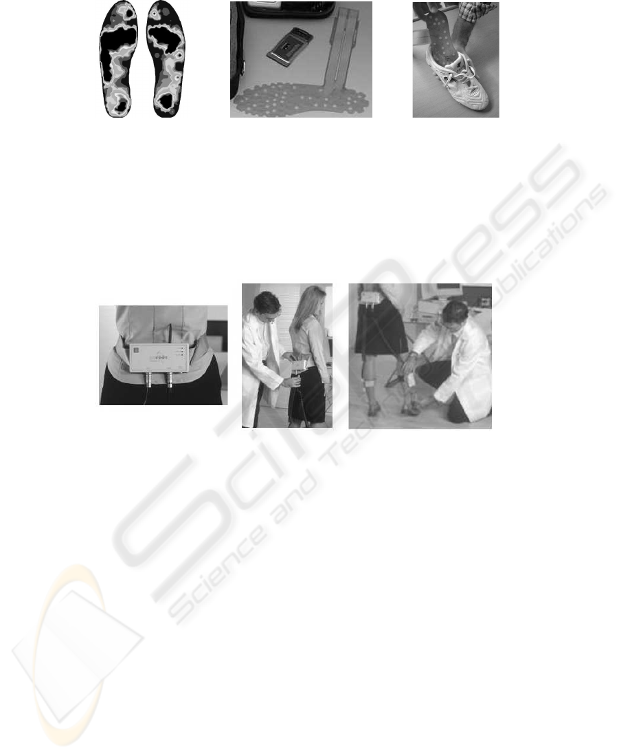
Fig.1. Example of pressures (left) and Biofoot
r
IBV Insole (center and right).
Biofoot
r
IBV allows the study of the foot pressures during the normal conditions,
walking and wearing shoes. Besides, by means of a telemetry system the signal is trans-
mitted wireless to a PC, where it is saved (figure 2). On the other hand, and in order to
avoid the effect in pressure values of the walking speed, two photocell barriers placed
at a known distance were used. This procedure permits the researchers to remove the
trials out of the interval [1,1.5] m/s, which defines the normal speed gait.
Fig.2. Biofoot
r
IBV Use.
In order to obtain a representative sample of the foot problems from a statistically
point of view, 60 subject of heterogeneous characteristics carried out the trials with
their usual footwear. A specialist in foot diseases classified them in different groups of
pathologies (a class label) after an exhaustive evaluation. Working in this way, for each
subject we obtain a labelled training vector. The pathologies diagnosed were:
– Rheumatoid arthritis.
– Pain in the heel or in other foot parts different of plant.
– Plantar foot pain.
– Hallus Valgus (bunion).
– Hemiplegia.
– Neuropathic foot.
– Degenerative problems of the Central Nervous System.
– Diabetic foot.
– Consequences of fractures.
Due to the high incidence of Pain in the heel or in other foot parts different of plant
and Plantar foot pain, and the fact that the 85% of the subjects were classified inside of
92

these groups, the study was only focused on these pathologies. Besides, in the database
the other pathologies has not a number of subject as great as representative for this
work. So, the used database is composed by 49 subjects, that is, 49 training vectors,
that are included in the two pathologies mentioned above (17 labelled subjects as “Pain
in the heel or in other foot parts different of plant” and 32 as “Plantar foot pain”).
4 Experiments
The experiments were carried out with the Biofoot
r
IBV database. Only two classes
were taken into account, as is mentioned above. The classification error of the proposed
method (LPD) is compared with the classification error of the well known k-NN rule
based on the Euclidean Distance. This error is estimated using the well known Leaving
One Out (LOO) estimation procedure due to the reduced number of available training
vectors. In LOO, given N labelled training vectors, two prototypes sets are built. In the
first one, called training set, we include N − 1 vectors and the other vector is included
(only it) in other set called test set. This process is repeated N times, each one including
a different vector in the test set and the others N − 1 in the training set. So, we do N
different experiments; each one with different training and test sets. In each experiment,
we train a classifier with the training set and test its performance with the test set. The
idea is to work as we did not know the real label of the test vector (that is; the real
pathology of the subject that corresponds with this vector) and see if the classifier is
able to find the class. The final result is the average over the N tests.
Results are shown in table 1. As can be seen, LPD results with reduced training
set and local weighted distances, are better than Euclidean Distance with the whole
training set results. The best result with LPD is obtained reducing the training set to
3 prototypes per class (14.3 % error rate), this result is a improvement of 20 % over
the best results obtained using k-NN with the Euclidean distance and all the training
prototypes (18.4 %). The LPD with a reduced set of the vectors is able to improve the
classification error in front of the original training set.
Table 1. k-NN error rate using Euclidean distance with different k values (left) and 1-NN LPD
error rate for different prototypes per class (right).
k Error Rate
1 18.4 %
2 18.4 %
3 28.6 %
4 24.5 %
5 40.8 %
Prototypes per class Error Rate
1 16.3 %
2 16.3 %
3 14.3 %
4 16.3 %
These results are still worse than those given by an expert, which obtains about 5%
error rate. This relative bad result of the automatic methods is due to the low num-
ber of samples available to learn adequately the class distributions. Also, the proposed
preprocessing step takes the average of all the pressures along the time loosing some
important temporal relations that are present in the plant during walking. We hope to
improve the error rate in future works with more training samples and the use of other
93

classification methods, as Hidden Markov Models (HMM), which allows us to treat the
foot plant pressures as a sequence of pressure vectors.
5 Conclusions and Future Work
A system to classify different foot pathologies, from pressure distribution over the foot
plant, has been presented. For this purpose, the Nearest Neighbor (NN) classification
rule using the Euclidean Distance and the NN classification rule improved by the LPD
method have been compared. The LPD obtained the best classification results with a
(14.3 % error rate), an 20% of improvement over the NN rule using the original train-
ing set and the Euclidean distance. Future work will focus on obtaining more samples
and using appropriate classification models (Hidden Markov Models) that allows us to
process the pressure of the foot plant as a temporal sequence of pressures.
References
1. Paredes, R., Vidal, E.: Learning prototypes and distances (lpd). a prototype reduction tech-
nique based on nearest neighbor error minimization. In: In ICPR 2004. (2004) 442–445
2. Paredes, R., Vidal, E.: Learning prototypes and distances: a prototype reduction technique
based on nearest neighbor error minimization. Pattern Recognition, Accepted (2005)
3. Kohavi, R., Langley, P., Y.Yung: The utility of feature weighting in nearest-neighbor algo-
rithms. In: Proc. of the Ninth European Conference of Machine Learning, Prague. Springer-
Verlag (1997)
4. Kononenko, I.: Estimating attributes: Analysis and extensions of relief. Technical report,
University of Ljubjana, Faculty of Electrical Engineering & Computer science (1993)
5. Wilson, D., Martinez, T.R.: Value difference metrics for continously valued attributes. In:
Proc. AAAI’96. (1996) 11–14
6. Howe, N., Cardie, C.: Examining locally varying weights for nearest neighbor algorithms.
In: Second International Conference on Case-Based Reasoning. springer (1997) 445–466
7. Paredes, R., Vidal, E.: A nearest neighbor weighted measure in classification problems. In
M.I. Torres, A.S., ed.: Proceedings of the VIII Symposium Nacional de Reconocimiento de
Formas y An
´
alisis de Im
´
agenes. Volume 1., Bilbao (1999) 437–444
8. Paredes, R., Vidal, E.: A class-dependent weighted dissimilarity measure for nearest neigh-
bor classification problems. Pattern Recognition Letters. 21 (2000) 1027–1036
9. Hastie, T., Tibshirani, R.: Discriminant adaptative nearest neighbor classification and re-
gressioon. Advances in Neural Informaton Processing Systems 8 (1996) 409–415 The MIT
Press.
10. Ricci, F., Avesani, P.: Data compression and local metrics for nearest neighbor classification.
IEEE Transactions on PAMI 21 (1999) 380–384
11. Short, R., Fukunaga, K.: A new nearest neighbor distance measure. In: Proc. 5th IEEE Conf.
Patter Recognition. (1980) 81–86
12. Peng, J., Heisterkamp, D.R., Dai, H.: Adaptative quasiconformal kernel nearest neighbor
classification. IEEE Transactions on Pattern Analysis and Machine Intelligence 26 (2004)
13. Paredes, R.: T
´
ecnicas para la mejora de la clasificacin por el vecino m
´
as cercano. PhD thesis,
DSIC-UPV (2003)
14. Paredes, R., Vidal, E.: Weighting prototypes. a new editing approach. In: Proceedings 15th.
International Conference on Pattern Recognition. Volume 2., Barcelona (2000) 25–28
15. Paredes, R., Vidal, E., Keysers, D.: An evaluation of the wpe algorithm using tangent dis-
tance. In: In ICPR 2002. (2002)
94
