Genetic Tuner for Image Classification

with Robotic Applications

Shahram Jafari and Ray Jarvis

Intelligent Robotics Research Centre (IRRC)

Monash University, VIC 3800, Australia

Abstract. This paper introduces a genetic tuner implemented for optimizing the

image scene analysis prior to the grasping of the objects, to realize a concrete

working robot named COERSU

. Firstly, different architectures of the adaptive

neuro-fuzzy inference system, multi-layer perceptron and K-nearest

neighborhood classifiers are compared to perform scene analysis and object

recognition. Following on, the MLP classifier is chosen due to its accuracy and

flexibility to be tuned by genetic algorithm. The real-time experiments (after

tuning) show that the performance of the genetically tuned MLP classifier is

improved in terms of accuracy due to this hybridization. Finally, snapshots of

the experimental results from COERSU in a table-top scenario to manipulate

some soft objects (e.g. fruit/egg) are provided to validate the methods.

1 Introduction

The context of the present research is a bigger effort to devise a multi-paradigm

model for robotic perception and manipulation. The major core is to integrate

different intelligent concepts to perform robotic eye-to-hand coordination and to

produce a working system, COERSU. How to make the robot decide based upon

information coming from different sensors, how to handle the feedback coming from

the dynamically changing environment and how to speed up the multi-paradigm

model of intelligence, are some of the high level questions that are attempted to be

answered during this research (Figure 1). Enabling COERSU to perceive, recognise

and manipulate soft objects on the table in a similar way to its human counterpart is

the most important part of this project.

The process of visual understanding includes image acquisition, segmentation

into coherent components, the recognition and pose determination of these

components and, potentially, an action plan related to the analysed environment. The

goal of image segmentation is to partition an image into meaningful homogeneous

regions [2, 6, 13]. The present research was based upon the critical assumption of

separating off-line tuning from the speed demanding real-time execution. Before,

during and after the scene analysis, different processes need to be performed, such as:

smoothing, registration, normalization and pseudo-colouring and segmentation.

An acronym for the Latin expression, “Cogito ergo sum” which means “I think

therefore I am”.

Jafari S. and Jarvis R. (2005).

Genetic Tuner for Image Classiﬁcation with Robotic Applications.

In Proceedings of the 1st International Workshop on Artiﬁcial Neural Networks and Intelligent Information Processing, pages 12-22

DOI: 10.5220/0001195100120022

 SciTePress

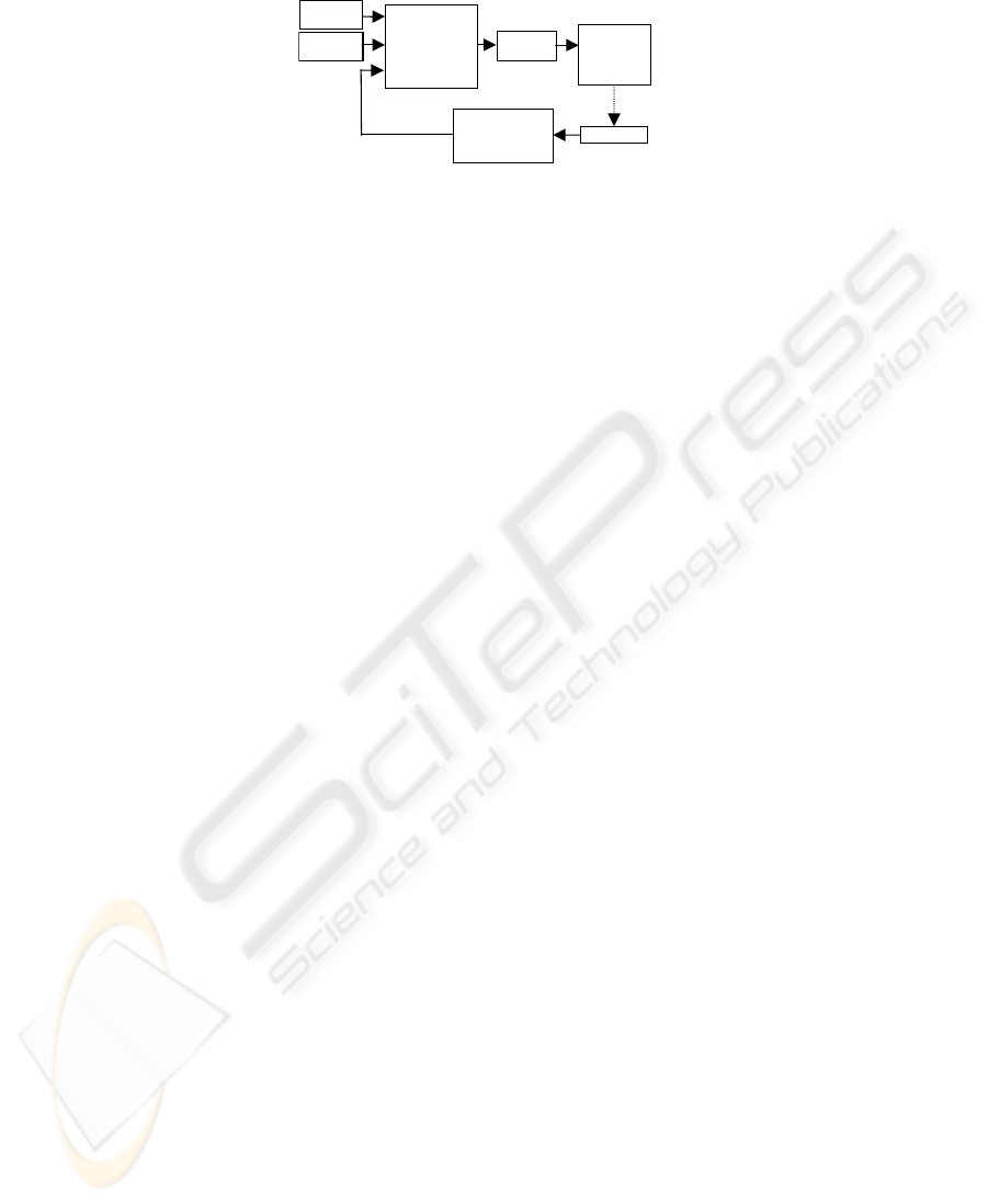
Genetically tuned

Segmentation,

ject recognitio

and Classification

RGB colour

information

Stereo range

information

Perception

and Control

Signals to the

actuator/mani

pulator of

neck and hand

Feedback from

human/environment:

Vision, Tactile,

Arm, Neck, User

Environment

edge detection,

Fig. 1. Block diagram of the working system.

For further details, refer to [9].

In this paper, Section 2 briefly explains scene analysis and compares different

methods for object recognition suitable for COERSU. The genetic tuner to optimize

the classifier is explained in Section 3. Snapshots of the video-clips are also shown at

the end to demonstrate the effectiveness of the methodologies.

2 Scene analysis

The major goal of scene analysis is to be able to determine what and where the

objects are in the scene, and the possible interrelationship between the objects in

order to manipulate them by a robot. There have been numerous studies of object

recognition in a robotic manipulation context. [3] developed an intelligent cruise

control (ICC). Object recognition based on sensor data was part of their intelligent

system and they made great contributions but mainly on car tracking systems, which

were far from our research problems. [4] proposed SENROB which detects and

manipulates objects within the working place of their robot, MANUTEC r2; however,

the camera is mounted in the robot’s hand which is quite different from our platform.

In our scene classification problem, the process was performed after the

segmentation and prior to the manipulation of the target object so that the robot arm

could not influence and disturb the classification of the objects. A five-nearest

neighbourhood classifier [7] was firstly considered because of its simplicity.

However, different neural network based methods were implemented to verify and

compare with the result of K-NN. We trained our system with fifty different known

object-pose cases. These consisted of five samples for each of ten prototype objects.

These objects were some foodstuffs such as, a banana, a cucumber, an egg, a kiwi

fruit, an eggplant, a capsicum and some other kitchen utensil: a mug, a plate, a spoon,

and a knife. Objects were chosen based on their simplicity for manipulation by a

robot hand with two fingers. For each of the objects we considered five different

samples/poses on the table in order to extract enough feature variations.

2.1 Classification features

The best combination of features will produce the greatest difference in the feature

values of significantly different shapes and the least difference for similar shapes.

The features used in our classification methods were chosen based on trial and error

and consisted of seven features for each segment found in the image after the

segmentation process: Perimeter, Area, Shape features A and B described below [7]

and Colour components (Red, Green, Blue).

The following two moment invariants are computed to achieve two goals:

primarily to get some shape descriptors, and secondly, to obtain scale, translation, and

rotation invariant features for the objects of interest.

0220

+=A

, (1)

()

0220

µµµ

+−=B

(2)

Where the central moments

used above (normalized with respect to

size) are obtained from the ordinary moments:

2/)2(

, (3)

()()

∑∑

−

−−=

),(

yxfyyxxv

, (4)

x =

y =

, (5)

∑∑

−

),(

yxfyxm

(6)

Where M,N: boundaries of the object rectangle

),( yxf

binary representation of the

object in the segmented image.

In order to have a measure of similarity between an unknown object and the

prototypes for K-NN classification, a weighted Euclidean distance metric was used

(1). Since the Euclidean distance function treats every dimension equally, it was

necessary to normalize the data. By analyzing all of the training data in a pre-

processing stage, we determined the range of every attribute and transformed the

entire dataset appropriately within the range of 0 and 1. Table 1 shows a typical

feature vector based on the image frame, its segmentation and edge detection for an

eggplant in a particular pose. Due to shape similarity between some of the objects

such as, banana, cucumber and eggplant, colour features discriminate better than

shape descriptors A and B, (2),(3).

Table 1. A typical feature vector for one pose of an eggplant.

No. Feature Name Feature values before

normalization

Normalized

feature value

3 Average RED

component

49.242537 0.193108

4 Average GREEN

component

52.514925 0.205941

5 Average BLUE

component

58.029851 0.227568

1 Shape descriptor A 0.326715 0.326715

2 Shape descriptor B 0.264920 0.264920

6 Area 268.000000 0.13958

7 Perimeter 89.000000 0.4635

2.2 Comparisons

Two types of each of the classifications were implemented: Two multi-layer

perceptron (MLP), K-NN (with K=1, K=5) and two ANFIS networks [12] were

implemented to compare the classification results. To keep the uniformity condition

and based on trial and error, all of the classifiers were trained with 50 known object-

pose cases, uniformly distributed between the samples, and tested with different 40

samples (4 samples for each of the ten classes of objects).

The first MLP classifier had a 7-5-1 structure where seven features, extracted

from the unknown object, were fed into the network as the inputs, a 5-neuron hidden

layer and one output with (0-9) values representing ten different classes of objects

(0.0 for the first class, 1.0 for the second… and 9.0 for the tenth class). However, in

the second network configuration, 10 different output neurons were considered based

on the idea that for each class of objects, only one output fires on (‘1’) and the other 9

output neurons present ‘0’s. In practice, the ideal (‘0’, ‘1’) outputs cannot be

obtained so we pick the maximum value of the ten outputs and its corresponding class

will be the predicted object. Both MLP’s were trained using error back-propagation

algorithm and a conventional sigmoid activation function was applied [11].

The parameters related to the ANFIS classifier are described as follows (Figure

2): A Takagi-Sugeno-Kang fuzzy rule-based system [15, 10] is equivalent to the

ANFIS network shown in Figure 2. Seven features of the unknown object are fed into

the network as the input layer. The output ranges from 0 to 9 and represents different

classes of the input. (e.g. class 0 represents mug, class 1 represents cucumber and so

on) and thirteen Sugeno type fuzzy rules were generated.

The confusion matrices [1] which contain information about actual and predicted

classifications were prepared for all of the classifiers using test cases.

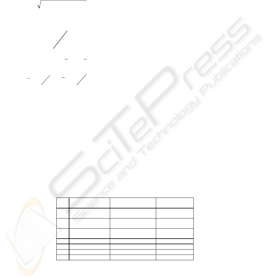
As an example (Table 2), after running the 5-NN algorithm, it classified the

objects in the scene correctly in 95% of the cases (38 samples). The accuracy was

calculated as the proportion of the total number of predictions that were correct. In

5% of the cases (2 samples), the system misclassified the ‘actual’ eggplant as a

‘predicted’ cucumber (Table 2). This is due to the similarity of the shapes of these

prototype objects in some poses and ‘outlier’ samples in the training set, addressed in

Section 3.

The result of the accuracy measurements for different methods, off-line training

time and on-line classification time for the image frames are provided in Table 3. The

on-line execution time is calculated as the time taken to analyze the whole image

frame (640 * 480 pixels). It can be observed in the comparison table (Table 3) that

there is a general trade-off between the execution time and the learning time for

different methods[8]. In other words, K-NN takes more time for real-time execution

but MLP and ANFIS perform faster for an unknown image and take more time for

the off-line training stage.

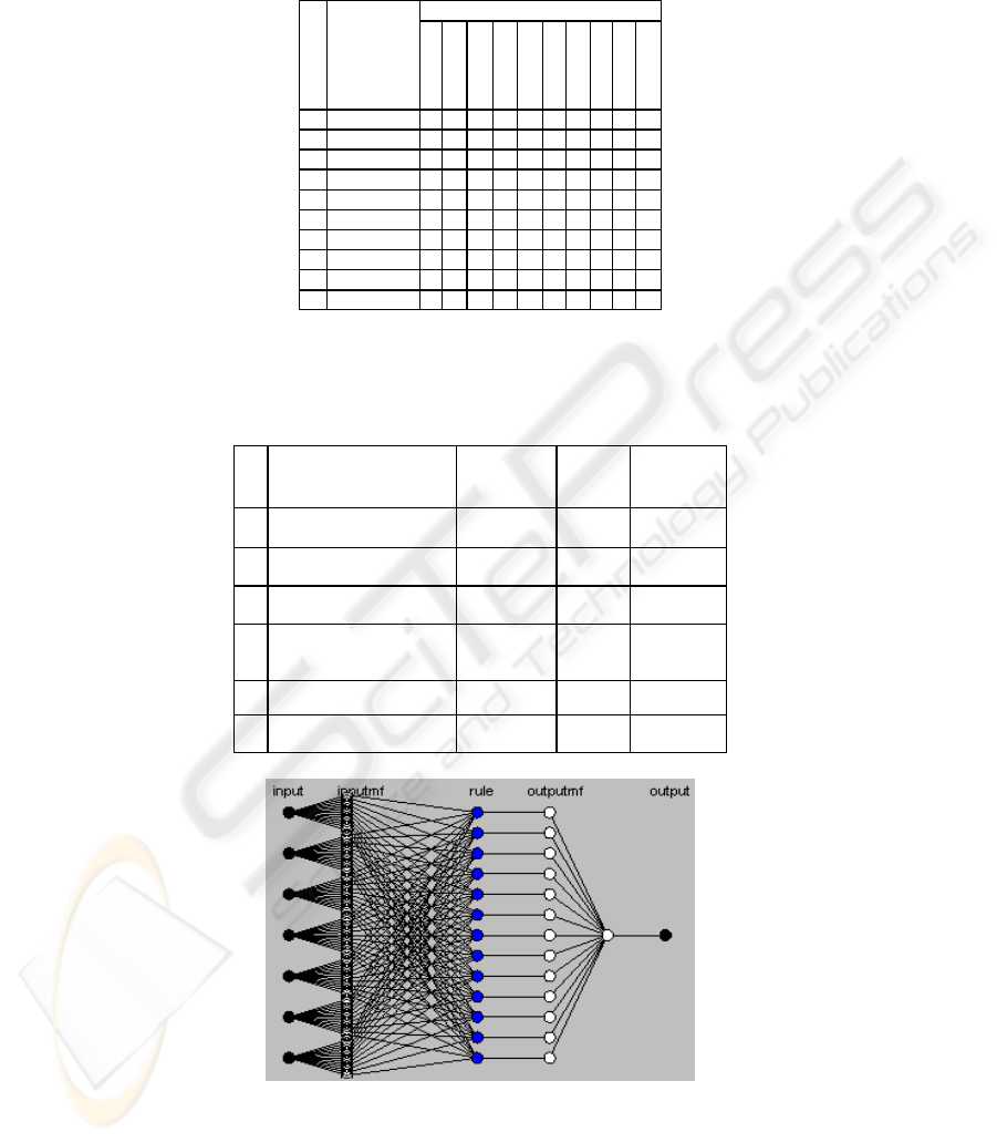
Table 2. Confusion matrix describing the performance of K-NN classifier. Correctly classified:

38 samples out of 40. Overall accuracy: 95%.

True class ( Actual)

No.

Classified as

(predicted)

Banana

Plate

Spoon

Knife

Mug

Cucumber

Eggplant

Egg

Kiwifruit

Capsicum

1 Banana

00 00 00000

2 Plate 0

0 0 0 0 0 0 0 0

3 Spoon 0 0

00 00000

4 Knife 0 0 0

0 0 0 0 0 0

5 Mug 0 0 0 0

00000

6 Cucumber 0 0 0 0 0

000

7 Eggplant 0 0 0 0 0 0

000

8 Egg 0 0 0 0 0 0 0

9 Kiwifruit 0 0 0 0 0 0 0 0

10 Capsicum 0 0 0 0 0 0 0 0 0

The 7-5-10 MLP showed a better performance than 7-5-1 MLP in terms of

classifying the noisy inputs. This can be attributed to the fact that the distribution of

the classification results was across a wider range of output neurons (10 instead of 1).

Table 3. Comparison between different methods

No.

Method

Learning

time (approx.

Sec.)

Accuracy

(%)

Execution

time (approx.

Sec.)

1 Nearest neighbourhood (1-

NN)

0 87.5% 15

2 5-nearest neighbourhood (5-

NN)

0 95% 20

3 Multi-layer perceptron (one

output) 7-5-1 layer structure

13 92.5% 10

4 Multi-layer perceptron (ten

output) 7-5-10 layer

structure

15 95% 12

NFIS (7 inputs, one output) 5 90% 15

6 Ten ANFIS (7 inputs, one

output)

28 92.5% 25

Fig. 2. ANFIS (7 inputs, 1 output) classifier.

3 Genetic tuner for MLP classifier

Since the supervised classifiers are highly dependent to the training sets, an

inaccurate measurement of the features of the training samples could result in a

misclassification. As discussed earlier in Section 2.1, seven essential features were

measured in order to extract the training samples. However, some features were

measured inaccurately and disturbed the classifier by appearing as severe outliers

which were inaccurate.

In contrast, according to Widrow’s rule of thumb [5] and trial and error, the noisy

training samples can help the classifier to have a better generalization [12]. However,

in this case the incorrect outliers were not genuine features of the training objects and

the classifier should not be generalized based on the incorrect information. These

wrong training samples were contributing to the error of the classification, especially

in the real-time mode, and needed to be removed from the training samples. The

consequence is that to get the best possible output from the classifier, it is necessary

to provide the system with significantly large number of non-conflicting training data.

The challenge is to distinguish between the correctly measured outliers among the

training samples (acceptable) and the incorrectly measured ones (not acceptable). The

incorrect training samples may only have one wrong feature value and the rest correct

but that one incorrect feature may drastically contribute to the error. The exhaustive

search for the selection of a suitable subset among the training samples could be quite

time-consuming, for example, using 50 samples will result in 2

different subsets.

In the literature, [14] utilized neural networks as outlier detector by suggesting a

rule to identify the “noise related” neurons. He further argues that little effort has

been reported in eliminating outliers prior to the training phase which affects the

results. However, his regression neural network could not be easily applied to the

classifier neural network. Current procedures for outlier detection such as using

Mahalanobis distance suffers from masking effect [14].

A Genetic algorithm was utilized in this paper to detect these incorrect outliers

and produce a subset of training samples that is suitable for the purpose of training

the classifier. Since all of the seven features were essential, the feature selection was

not included in the genetic tuner although it could be potentially performed.

Collaboration between GA and neural networks has been reported in the literature

before. [16] devised genetic neural networks for classification of remotely sensed

images. The architecture of the neural network was designed using GA which makes

it different from our problem.

3.1 Implementation details of the MLP genetic tuner

The aim of this genetic tuner was to optimize the neural network classifier by

selecting a suitable subset of the training samples and removing the dubious values to

train the network. The importance of the tuning is that the final correct subset of the

training samples can be applied to other classification methods as well and it

decreases the computation time of the real-time execution (for K-NN methods) or the

learning time (for neural network based methods) by removing the dubious values.

Therefore, the mapping between the samples space and genetic space was generated

by considering the chromosome to have the same number of genes as the training

samples, in this case 50.

The genes were holding a binary value showing whether the corresponding

training sample exists in the subset (“1”) or not (“0”). Therefore the conventional

genetic functions could be applied plus a trivial constraint. The minimum allowable

number of training samples for each object was considered as a threshold so that at

least one training sample exists for each of the object classes.

It was decided, based on trial and error, that the genetic algorithm have a

population size of 20 chromosomes for each generation and a maximum number of

200 generations for evolution at each run to guarantee the optimum solution. The

roulette selection of the parent was considered for the replication and the mutation

probability of 0.1 and cross-over probability of 0.5 were chosen. Elitism in choosing

the offspring generation was considered as well.

3.1.1 Chromosome fitness evaluation

For the MLP genetic tuner, the goal is to evolve the chromosomes to maximize the

following Fitness(i):

()

2211

)()(

)(

ifwifw

iFitness

×+

(7)

()

)(1

)(

iMSE

(8)

()

iMSE

tki

actual

tki

desired

−

∑∑

==11

),,(),,(

)(

(9)

()

)(1

)(

iMisclass

(10)

∑

iMisclass set test in the icationsmisclassif)(

(11)

Where i is the chromosome, f

is the fitness measured related to the mean squared

error (MSE) between the actual and the desired output in the training data, MSE(i), is

the mean-squared error for chromosome i; T, number of test samples, N, number of

objects, w1and w2, weights assigned to partial fitness f

and f

, , M, number of

training samples, k, the neuron in the output layer,

),,( tki

desired

, the desired output for

neuron k for a particular training sample t, in chromosome i,

),,( tki

actual

o , the actual

output of the classifier, f

, the fitness measured related to the misclassification of an

accurate test sample, ‘+1’ avoids divide by zero in the fitness equations.

In order to obtain a balance between two criteria for the fitness measurments, we

decided to utilize such a weighted averaging fitness. The fitness function was a

compromised estimation between the error in misclassification of the test samples and

the mean squared error between the actual output and the ideal one for the training

data.

The test samples were gathered based on unseen objects different from the

training samples in terms of both the physical shape and pose of the object on the

table. For each fitness measurement, MLP classifier is trained using the conventional

error-backpropagation algorithm.

3.2 Experimental results

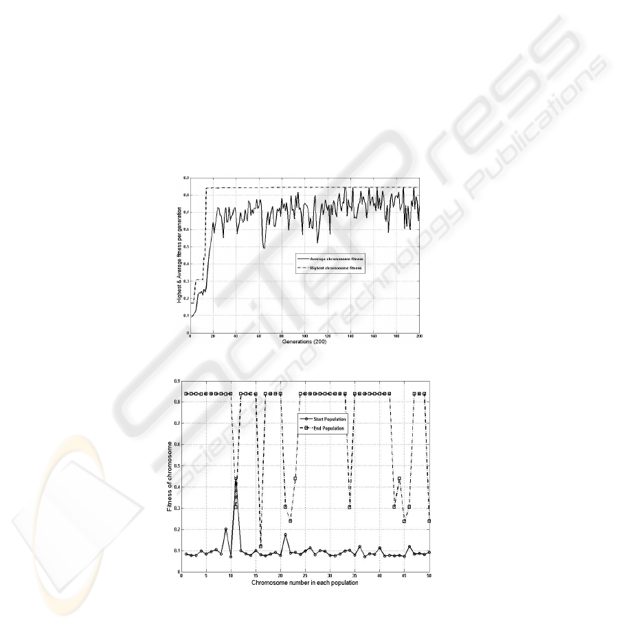
After running the genetic algorithm up to 200 generations a few times, and assuming

the following parameters in the equations (7-11): M=50, N=10, T=40, w

= 1, w

= 4

(based on trial and error), Figure 3 shows the elite chromosome fitness (highest

fitness) and average fitness for each generation. It can be observed that the average

fitness gradually converges to the maximum fitness found.

Also, fitness of start population versus end population for 200 generations is shown

in Figure 4. It is observed that the end population has much fitter chromosomes than

the start population.

The elapsed time to complete the whole process of tuning the classification with

the above configuration was 3896 Sec. (65 minutes) on an ordinary 1.60 GHZ PC.

This is acceptable, especially because the process was performed off-line prior to the

production mode.

Fig. 3. Highest and average fitness for 200 generations

Fig. 4. Fitness of start and end populations for 200 generations.

3.3 Final Configuration of the Real-Time Pattern Classifier (Combination

Strategy)

In order to make a more powerful classifier, compensate the deficiencies of each one

and increase the performance of the whole system in terms of reliability, combination

of different classifiers is preferred.

In practice, the problem with a fixed test set is that the classifier becomes rigid

by tuning itself based on a fixed set of test samples. Therefore, it was decided to take

an odd number of correct test sets (for our case we chose 3 sets) and use each of them

to extract the corresponding suitable training subset and consequent classifier.

Therefore, each of the MLP classifiers was slightly different from the others. During

the production mode, in order to find a compromised solution between the decisions

of the different classifiers, the voting mechanism was implemented so that the class

of object which had the majority of approval was selected as the final result, as

shown in Figure 5. (If three of the classifiers predicted differently, the object would

remain unknown, however, this case did not happen in our experiments).

Finally, Figures 6, 7 show the snapshots of the integration of the processes, from

the on-line observation to the grasping of an egg.

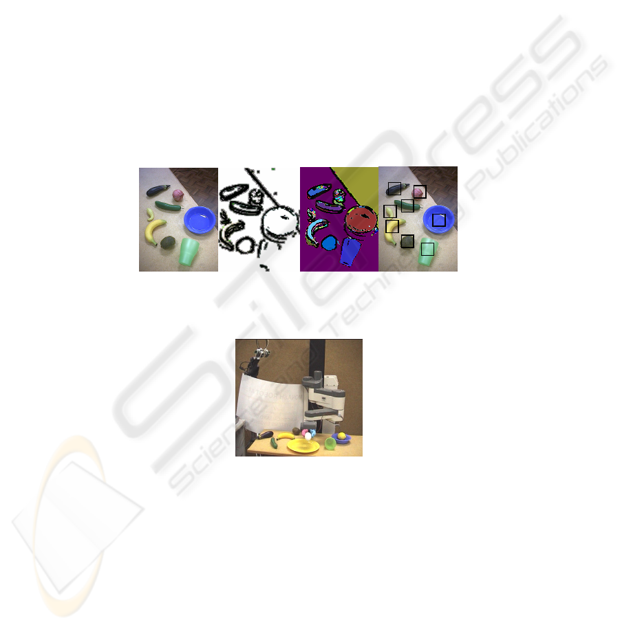
Fig. 5. Result of online scene analysis (from left to right): (a) original image frame (b) result of

edge detection (c) segmentation based on the genetically tuned parameters (d) genetically

tuned object classification.

Fig. 6. An egg is grasped and picked up by COERSU in a table-top scenario.

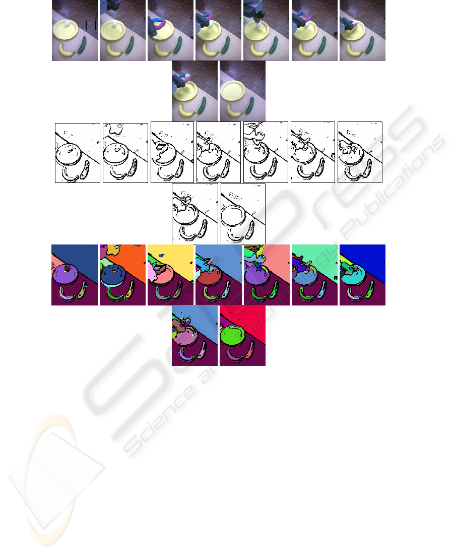
Fig. 7. On-line result in response to the command: ‘Grasp the egg’ (column-wise from left)

a) Frame No.1-initial scene, objects are recognized b) Frame No.2- first positioning of the

tooltip c) Frame No.8- alignment with the centroid of the target d) Frame No.9- 3D x, y

adjustments e) Frame No.10- target verification f) Frame No.11- opening the tooltip g)

Frame No. 12- wrist tilt and grasping the egg h) Frame No. 13- final grasping, tilt back the

wrist i) Frame No. 14- ready for the next command. (row-wise from top) i) original image

ii) result of edge detection iii) tuned segmentation.

4 Conclusions

The result of the scene analysis and classification using different architectures of the

classifiers (Multi-layer Perceptron, ANFIS and K-NN classifiers) were compared. A

genetic tuner for optimizing the multi-layer perceptron classifier was explained to

support image scene analysis for our robotic platform, COERSU. Although using the

tuner makes the system more complicated, it is preferable to apply it to obtain higher

degrees of precision and real-time execution.

References

1. Del Frate, F., G. Schiavon, D. Solimini, et al. 2003, "Crop classification using

multiconfiguration C-band SAR data." Geoscience and Remote Sensing, IEEE

Transactions on, vol. 41(7): 1611-1619.

2. Gong, M. and Y. H. Yang 2001, Genetic-Based Multiresolution Color Image

Segmentation. in Vision Interface 2001, Ottawa, Ontario.

3. Handmann, U., I. Leefken, C. Tzomakas, et al. 1999, A flexible architecture for intelligent

cruise control. in Intelligent Transportation Systems, 1999. Proceedings. 1999

IEEE/IEEJ/JSAI International Conference on: 958-963.

4. Hartmann, G., S. Drue, J. Dunker, et al. 1994. The SENROB vision-system and its

philosophy. in Pattern Recognition, 1994. Vol. 2 - Conference B: Computer Vision &

Image Processing., Proceedings of the 12th IAPR International. Conference on. vol. 2:

573-576 vol.2.

5. Haykin, S. 1994, Neural networks: A comprehensive Foundation, Macmillan.

6. Hofman, I. D. 2000, Three dimensional scene analysis using multiple view range data. in

Intelligent Robotics Research Centre (IRRC). Clayton, Monash University, Australia.

7. Hu, M.-K. 1962, "Visual pattern recognition by moment invariants." Information Theory,

IEEE Transactions on, vol. 8(2): 179-187.

8. Jafari, S. and R. A. Jarvis 2003, A Genetic Off-line Tuner for Robotic Humanoid Visual

Perception presented at IEEE International Congress on Evolutionary Computation (CEC-

2003).

9. Jafari, S. and R. A. Jarvis 2005, "Robotic Hand Eye Coordination: From Observation to

Manipulation (invited paper under review, Submission date: March 2005)." International

Journal of Hybrid Intelligent Systems(special issue).

10. Jafari, S., R. A. Jarvis and T. Sivahumaran 2004, Hybrid Intelligent Models for Visual

Servoing presented at IEEE Conference on Cybernetics and Intelligent Systems (CIS),

Singapore.

11. Jafari, S., F. Shabaninia and P. A. Nava 2002, Neural network algorithms for tuning of

fuzzy certainty factor expert systems presented at IEEE/WAC World Automation Congress,

USA.

12. Jang, J.-S. R. 1993, "ANFIS: adaptive-network-based fuzzy inference system." Systems,

Man and Cybernetics, IEEE Transactions on, vol. 23(3): 665-685.

13. Le Moigne, J. 1992, Refining Image Segmentation by Integration of Edge and Region Data

VO - 2, vol. 2.

14. Lopez, C. 1999, Looking inside the ANN "black box": classifying individual neurons as

outlier detectors presented at Neural Networks, 1999. IJCNN '99. International Joint

Conference on.

15. Negnevitsky, M. 2002, Artificial Intelligence: A Guide to Intelligent Systems 1/e. Adison

Wesley: 394.

16. Sasaki, Y., H. de Garis and P. W. Box 2003, Genetic neural networks for image

classification presented at Geoscience and Remote Sensing Symposium, 2003. IGARSS

'03. Proceedings. 2003 IEEE International.