
Structural Persistence of Three Dimensional
Autonomous Formations
Changbin Yu
1
, Julien M. Hendrickx
2
, Barıs¸ Fidan
1
and Brian D.O. Anderson
1
1
National ICT Australia Ltd. and
Research School of Information Sciences & Engineering, the Australian National University,
216 Northbourne Ave., Canberra ACT 2601 Australia
2
Department of Mathematical Engineering, Universit
´
e Catholique de Louvain,
Avenue Georges Lemaitre 4, B-1348 Louvain-la-Neuve, Belgium
Abstract. Built upon a recently developed theoretical framework, we consider
some practical issues raised in multi-agent formation control in three dimensional
space. We introduce the partial equilibrium problem, which is associated with
unsafe control of a formation in practical 3-dimensional applications. We define
structurally persistent graphs, a class of persistent graphs free of any partial equi-
librium problem. In real deployment of control of multi-agent systems, forma-
tions with underlying structurally persistent graphs are of interest. We study the
connections between the allocation of degrees of freedom (DOFs) across agents
and the characteristics of persistence and/or structural persistence of a directed
graph. We also show how to transfer degrees of freedom between agents, when
the formation changes with new agent(s) added, to preserve persistence and/or
structural persistence.
1 Introduction
In [1], we have generalized the definition of persistence to ℜ
d
for d ≥ 3, seeking
to provide a theoretical framework for real world applications, which often are in 3-
dimensional space as opposed to the plane. We also have derived some new properties of
persistent graphs and given an operational criterion to determine if a graph is persistent.
In this paper, we demonstrate that a persistent formation, as defined in [1], may also
⋆ ⋆ ⋆
The work of Brian D.O. Anderson,Barıs¸ Fidan and Changbin Yu is supported by National ICT
Australia, which is funded by the Australian Government’s Department of Communications,
Information Technology and the Arts and the Australian Research Council through the Back-
ing Australia’s Ability Initiative. Changbin Yu is an Australia-Asia Scholar supported by the
Australian Government’s Department of Education, Science and Training through Endeavours
Programs.
†
The work of Julien M. Hendrickx is supported by the Belgian Programme on Interuniversity
Attraction Poles initiated by the Belgian Federal Science Policy Office, and by the Concerted
Research Action (ARC) “Large Graphs and Networks” of the French Community of Belgium.
The scientific responsibility rests with its authors. Julien M. Hendrickx is a FNRS (Belgian
Fund for Scientific Research) fellow.
Yu C., M. Hendrickx J., Fidan B. and D.O. Anderson B. (2005).
Structural Persistence of Three Dimensional Autonomous Formations.
In Proceedings of the 1st International Workshop on Multi-Agent Robotic Systems, pages 47-55
DOI: 10.5220/0001194600470055
Copyright
c
SciTePress

suffer from a practical problem where each agent can move to a position which satisfies
the constraints on it once all the other agents are fixed but it is not possible to satisfy all
the constraints on all the agents at the same time.
In Section 2, we formally characterize the above problem, which we call the partial
equilibrium problem, and which is closely associated with unsafe control of a forma-
tion in practical 3-dimensional applications. We then introduce the definition of a struc-
turally persistent graph, a class of persistent graphs free of any partial equilibrium prob-
lem. In real deployment of control of multi-agent system, formations with underlying
structurally persistent graphs are of interest. It is established in Secction 2 incidentally
that in two dimensions, structural persistence and persistence are equivalent.
In Section 3, we focus on the connections between allocation of degrees of freedom
(DOFs) across agents and the characteristics of persistence and/or structural persistence
of a directed graph. We also show how to transfer degrees of freedom between agents,
when the formation changes with new agent(s) added, to preserve persistence and/or
structural persistence. We study cycle-free graphs in ℜ
3
and show some more powerful
results that exist in this special case, such as the existence of a quadratic time criterion to
verify the cycle-free property and to decide persistence, which automatically guarantees
structural persistence.
We end the paper with concluding remarks in Section 4. Note that all the proofs are
omitted due to space limitations. However, a full version of this work together with the
campanion paper [1] is available in preprint from the authors.
2 Partial Equilibrium Problem and Structurally Persistent
Graphs
Consider a persistent graph G = (V, E) in ℜ
d
(d ∈ {2, 3, . . .}). The partial equilibrium
problem we want to avoid is the following: There is a subset
˜
V ⊂ V of vertices such
that all the vertices in
˜
V are at fitting positions whatever the positions of the vertices
in V \
˜
V are, but there exists no position assignment for the vertices in V \
˜
V such that
the whole representation is fitting. For example, consider the 3-dimensional persistent
graph
¯
G shown in Figure 1, an associated set
¯
d of desired lengths d
ij
> 0 for all the
edges
−−→
(i, j), and a realization ¯p of
¯
d in agreement with Figure 1. Identify
˜
V with {1, 2}.
Since the vertices 1 and 2 have zero out-degrees, they are at fitting positions for any
representation of the graph, whatever the positions of 3, 4, 5 are. However, there are
representations of
¯
G arbitrarily close to ¯p where the vertices 3, 4, and 5 cannot be at
fitting positions at the same time. From the perspective of formations, in the formation
represented by
¯
G, there exist two leaders, 1 and 2, which are allowed to move freely in
ℜ
3
without any constraint. This freedom, however, makes it impossible in some cases
for the agents 3, 4, and 5 to meet all the distance constraints on them, although
¯
G is
persistent, according to the definition given in Section 3 of [1]. In such a case, we will
say that
¯
G is in partial equilibrium.
The existence of such partial equilibrium problems in three and higher dimensional
spaces makes it necessary to analyse persistent graphs further and introduce new con-
cepts such as structural persistence that will be defined in this section. In ℜ
2
, how-
ever, there is no persistent graph suffering from partial equilibrium problems, as ex-

1
2
3
4
5
Fig.1. A persistent graph in ℜ
3
which is not structurally persistent.
plained later in Theorem 1. Let us consider a persistent graph G = (V, E) in ℜ
d
(d ∈ {2, 3, . . .}) with a representation p. Let
¯
d be the set of distances corresponding
to p. G is in partial equilibrium, and thus has the partial equilibrium problem if there
exists a non-empty vertex subset
˜
V ⊂ V , a constant ε > 0 and a mapping p
¯ε
indexed
by ¯ε,
n
p
¯ε
:
˜
V → ℜ
d
|0 < ¯ε ≤ ε
o
such that for any ¯ε ≤ ε the following hold:
1. d(p(i), p
¯ε
(i)) ≤ ¯ε, ∀i ∈
˜
V .
2. For all i ∈
˜
V , p
¯ε
(i) is a fitting position with respect to
¯
d, irrespective of the posi-
tions of the vertices in V \
˜
V .
3. There exist no fitting representation p
′
: V → ℜ
d
in B(p, ¯ε)
∆
=
¯p : V → ℜ
d
|d(p, ¯p) ≤ ¯ε
,
with respect to
¯
d, such that p
′
(i) = p
¯ε
(i), ∀i ∈
˜
V .
If a persistent graph is not in partial equilibrium, it is called a structurally persistent
graph. To analyse this concept further, it is defined that for a given directed graph G =
(V, E), a subgraph G
′
= (V
′
, E
′
) is a practically closed subgraph of G if for any vertex
i ∈ V
′
, d
+
G
′
(i) ≥ min{d, d
+
G
(i)}, where d
+
G
′
(i) denotes the number of outgoing edges
incident to the vertex i of a graph G
′
. We remark that a closed subgraph is always a
practically closed subgraph, since each vertex of it satisfies the criterion defined above.
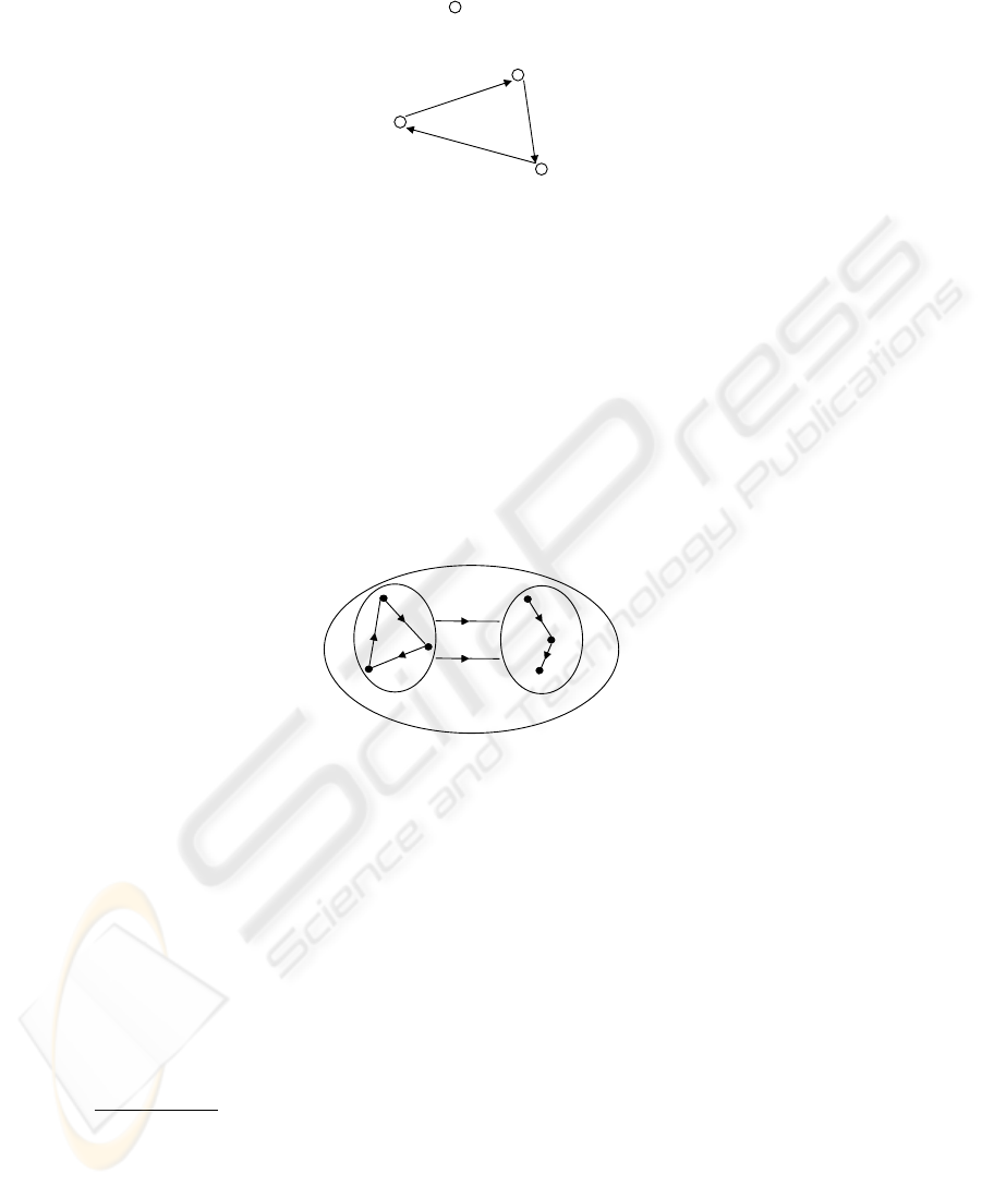
In the 2-dimensional example shown in Figure 2, where V
′
= {1, 2, 3}, G
′
is a
practically closed subgraph of G but not a closed subgraph of G. All the outgoing edges
of 1 and 2 in G remain in the subgraph G
′
. Vertex 3, on the other hand, has two outgoing
edges in G
′
(making G
′
a practically closed subgraph) and another one not in G
′
. From
a perspective of formations where vertices denote agents and edges denote awareness,
in G, although 3 is aware of 4, it may not be able to react to correctly maintain its
distance from 4 because its position is locked by the constraints with respect to the
vertices 1 and 2.
The relation between partial equilibrium problems and practically closed subgraphs
is examined in the following propositions.
Proposition 1 Consider a persistent graph G = (V, E) in ℜ
d
(d ∈ {2, 3, . . .}) with a
representation p and a set
¯
d of distances corresponding to p. Let G
′
= (V
′
, E
′
) be a
subgraph of G where V
′
is a non-empty vertex subset of V . Then, G
′
is a practically
closed subgraph of G if and only if there exist a constant ε > 0 and a mapping p
¯ε
indexed by ¯ε,
p
¯ε
: V
′
→ ℜ
d
|0 < ¯ε ≤ ε , p
¯ε
is the restriction of p → V
′
such that
for any ¯ε ≤ ε the following hold:

1
2
3
4
1
2
3
4
G
G’
Fig.2. A practically closed subgraph in ℜ
2
.
1. d(p(i),p
¯ε
(i)) ≤ ¯ε, ∀i ∈ V
′
, for all p
¯ε
in the mapping set.
2. For all i ∈ V
′
, p
¯ε
(i) is a fitting position with respect to
¯
d, irrespective of the
positions of the vertices in V \V
′
.
Proposition 2 Consider a persistent graph G = (V, E) in ℜ
d
(d ∈ {2, 3, . . .}) with a
representation p and a set
¯
d of distances corresponding to p. G is structurally persistent
if and only if every non-empty practically closed subgraph of G is persistent.
The following theorem, which uses Proposition 2, states that there is no partial
equilibrium problem in ℜ
2
, as mentioned in the beginning of the section.
Theorem 1 Any persistent graph G ∈ ℜ
2
is structurally persistent and has all its
practically closed subgraphs persistent.
Proposition 2 states that a graph is not structurally persistent if and only if it contains
a practically closed subgraph that is not persistent. Development of this notion leads to
the following proposition, which gives another necessary and sufficient condition for a
persistent graph to be structurally persistent.
Proposition 3 Let G = (V, E) be a persistent graph in ℜ
d
. G is structurally persistent
if and only if there is no non-persistent closed subgraph of G with less than d vertices.
The following corollary, which is a major result of the section, and which immedi-
ately follows from Proposition 3, gives a more explicit necessary and sufficient condi-
tion for 3-dimensional persistent graphs to be structurally persistent. It also gives more
insight for the problem encountered in the example in Figure 1.
Corollary 1 A persistent graph G = (V, E) in ℜ
3
is structurally persistent if and only
if there is at most one leader
3
in G.
Remark 1 For some dimensions d > 3, one can have a non-persistent closed subgraph
with less than d vertices in a graph that has only one leader. An example in ℜ
6
is shown
in Figure 3. In general, in a given d-dimensional persistent graph, the presence of a
non-persistent closed subgraph can be checked by looking only at the vertices with out-
degree less than d − 1, which are finite in number because of the bound on the total
DOF count.
6-DOF
5-DOF
5-DOF
5-DOF
Fig.3. A non-persistent closed subgraph in ℜ
6
that does not have two leaders. Note that in ℜ
6
,
the total DOF count of a persistent graph can be up to 21.
Remark 2 In contrast to the case d = 3, for d ≥ 4, a non-persistent closed subgraph of
a persistent graph can be connected. Consider, for example, the 4-dimensional directed
graph G = (V, E) shown in Figure 4. G is constraint consistent because no vertex has
an out-degree larger than 4. Moreover, it is minimally rigid and it can be obtained by
removing an edge from the complete graph K
6
, which is trivially rigid. On the other
hand, the closed subgraph G
2
of G is non-rigid and hence non-persistent. Therefore, G
is not structurally persistent. Note that G
2
is connected although it is non-persistent.
all possible
edges from
G1 to G2
M
G1
G2
G
Fig.4. A 4-dimensional persistent graph with a non-persistent and connected closed subgraph.
3 Allocation of DOFs in ℜ
3
and Trilateration
In Section 2, we have seen that for a directed graph, persistence is not enough to avoid
partial equilibrium problems. In the following subsections, we study how the way de-
grees of freedom happen to be allocated to the vertices of a directed graph is a key de-
terminant of the structural persistence or otherwise of that graph. In an application sce-
nario, this corresponds to giving/restricting the autonomy of certain agents (abstracted
as degrees of freedom of vertices) of the formation [2].
3
An agent is a leader if it has no constraints on its movement, e.g. in Figure 1, both agents
represented by vertices 1 and 2 are leaders. In associated graphs, corresponding vertices have
no outgoing edges.

3.1 DOF Allocation and Transfer via Directed Trilateration in ℜ
3
In this section, we study the properties of the directed version of Henneberg-like vertex
addition in 3 and higher dimensions, which is an abstraction of the event that new
agents join a formation, one at a time. We give examples of applying such operations to
manipulate DOF allocation of persistent graphs, in particular, in ℜ
3
.
Let us consider a persistent graph G = (V, E) in ℜ
d
(d ∈ {2, 3, . . .}) where |V | ≥
d. A directed d-vertex addition, DVA (d, n) where n ∈ {0, . . ., d}, transforms G to
another persistent graph G
′
= (V
′
, E
′
) where V
′
= V ∪ { i }, E
′
= E ∪ {
−−−→
(i, k) :
∀k ∈ V
1
} ∪
−−→
(j, i) : ∀j ∈ V
2
}, V
1
, V
2
⊆ V , V
1
∩ V
2
= ∅, |V
1
| = d − n , |V
2
| = n
, and DOF (j) ≥ 1 , ∀j ∈ V
2
,
4
provided that the vertices of V
1
∪ V
2
do not lie in any
q-dimensional hyperplane where q < d.
We note that from Lemma 2 of [1], constraint consistency is preserved with the
directed d-vertex addition defined above. Moreover, from the following lemma which
is drawn from [3,4], we see that the rigidity is also preserved.
Lemma 1 [3, 4] A graph obtained by adding one vertex to a graph G = (V, E) in ℜ
d
and d edges from this vertex to other vertices of G is rigid if and only if G is rigid.
Hence by Theorem 2 of [1], the graph obtained after applying a directed d-vertex
addition on a persistent graph in ℜ
d
is persistent, i.e., the d-directed vertex addition
defined above preserves the persistence of the graphs.
Remark 3 Consider a persistent graph G = (V, E) in ℜ
d
. Let G’ = (V’, E’) be the graph
obtained by applying the operation DVA(d,n) to G, where V’=V ∪ {i}. Then we have:
DOF
G
′
(i) = n ; DOF
G
′
(j) ≤ DOF
G
(j), ∀j ∈ V. and DOF
G
(j) − DOF
G
′
(j) ∈
{0, 1} , ∀j ∈ V.
In the remaining part of this section, we only consider ℜ
3
, although results can
be easily expanded to higher dimensions. As a more convenient nomenclature in ℜ
3
,
we use the term directed trilateration operation, abbreviated DT(·), DT(n) in place of
directed 3-vertex addition or DVA(3, n).
An undirected graph formed by a sequence of trilateration operations starting with
an initial undirected triangle, often called a trilateration graph, is guaranteed to be
generically rigid in ℜ
3
and globally rigid in ℜ
2
. A trilateration graph can always be con-
structed/deconstructed using a polynomial time algorithm, where a reverse trilateration
can be performed by removing a vertex with degree 3 at each step. Note that a seed with
3 vertices is needed to initiate a trilateration sequence. However, two different directed
triangular seeds can start a directed trilateration operation in ℜ
3
as defined in Figure
5(a) and Figure 5(b) are called the leader-first follower-second follower (L−F F −SF )
and the balanced triangle (B
1
B
2
B
3
) seeds, respectively.
Remark 4 The leader-first follower-second follower seed is analogous to the leader-
follower structure defined for a 2-dimensional cycle-free graph [5]. The set of DOF
counts of the seed vertices is {3 ,2 ,1}. The balanced triangle is nothing more than a
directed triangle (cycle) in a cyclic graph and the corresponding DOF count set is {2
,2 ,2}.
4
Non-existence of V
2
means the corresponding DVA(n) cannot be performed for the graph.

L
FF
SF
B
1
B
2
B
3
(a) (b)
Fig.5. The two directed triangular seeds.
Specifically in the application to 3 dimensional agent formations, note the meanings
of the DT(i) operation for different i can be interpreted as follows,
– DT(3) means election of a new leader.
– DT(2) may result in either breaking/restoring the balanced control structure, or
election of a new first-follower.
– DT(1) may also result in either breaking/restoring the balanced control structure at
more a detailed level, or creation/change of second follower.
– DT(0) preserves the control structure and no decision has to be made by pre-
existing agents.
Noting that in a 3-dimensional persistent graph, there are at most 6 DOFs (as op-
posite to 3 DOFs in the ℜ
2
case) to be allocated among the vertices, we can list the
following six types of DOF allocation (abbreviated DOF allocation state S
1
to S
6
with
DOF counts of vertices):
– S
1
= {3, 2, 1, 0, 0, . . .} , S
2
= {2, 2, 2, 0, 0,. . .}
– S
3
= {3, 1, 1, 1, 0, 0, . . .} , S
4
= {2, 2, 1, 1, 0, 0,. . .}
– S
5
= {2, 1, 1, 1, 1, 0, 0,. . .} , S
6
= {1, 1, 1, 1, 1, 1, 0, 0,. . .}
Further, we define a transient type of DOF assignment S
0
= { 3, 3, 0, 0, . . .}, which
can (only) be obtained by applying a DT(3) operation to S
3
. S
0
is named “transient”
because it apparently allows two leaders simultaneously in control of a formation, and
hence this creates instability and we want the DOF assignment to avoid this state. Recall
that the underlying directed graph of such a formation is a persistent graph with a partial
equilibrium problem, i.e. it is persistent but NOT structurally persistent (An example of
a graph that is in transient state S
0
can be seen from Figure 1).
We study the transformational relationship between the possible distribution of
DOFs by applying the appropriate DT(·) operation using the “state transition diagram”
shown in Figure 6. We have the following observations:
– Starting from any one of the two directed triangular seeds, we can build any graph
with any of S
0
- S
6
by adding at most three vertices using directed trilateration.
– Any desired DOF reallocation pattern(with no allocation to a specific vertex) can
be achieved by at most four directed trilaterations starting with any of the six types
of DOF allocation.
– Any desired stable DOF reallocation pattern can be achieved by at most three di-
rected trilaterations starting with any stable DOF allocation.
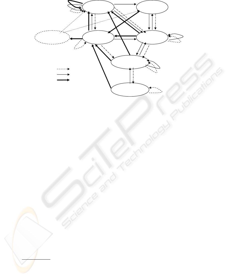
3, 2, 1, 0, 0… 2, 2, 2 , 0, 0…
3, 1, 1, 1, 0, 0 … 2, 2 , 1 ,1, 0 , 0…
2, 1, 1, 1,1, 0, 0…
1,1, 1 ,1 ,1,1, 0, 0…
3, 3, 0, 0 …
Legend:
DT(1)
DT(2)
DT(3)
Fig.6. The state transition diagram for directed trilaterations.
The observed results above gives an upper bound on the number of agents required
in order to perform a system reconfiguration operation, such as replacement or elimina-
tion of leaders/first-follower/second-follower, or change to balanced cooperative control
of 3 leaders. And it also gives the possible consequences in a closing ranks problem
5
,
where the lost agent has a certain positive number of DOFs .
3.2 Cycle-Free Graphs
Persistence of cycle-free graphs in ℜ
2
was studied in [5]. In this section, we derive a
simple criterion to decide the persistence and structural persistence of cycle-free graphs
in ℜ
d
. We also show an explicit way to build all the persistent cycle-free graphs.
Proposition 4 A graph obtained by adding one vertex to a graph G = (V, E) in ℜ
d
and
at least d edges leaving this vertex is persistent if and only if G is persistent.
We thus know that a cycle-free graph obtained by successively adding vertices all
with out-degree d, i.e. DVA(d,0), to an initial seed of a cycle-free persistent graph con-
taining only d vertices is persistent.
Next,we focus on cycle-free persistent graphs in ℜ
3
, which have important applica-
tion in safe control of multi-agent formations.
5
The closing ranks problem for a given rigid formation which has lost a single agent, is to
find new links between some agent pairs which, if maintained cause the resulting formation to
again be rigid.

Theorem 2 A cycle-free graph in ℜ
3
having more than 2 vertices is persistent if and
only if it has a closed subgraph which is the leader-first follower-second follower trian-
gle, and every other vertex has an out-degree larger than or equal to 3.
Moreover, every cycle-free persistent graph in ℜ
3
can be obtained from an original
seed composed by the leader-first follower-second follower by adding vertices one by
one in the way described in Proposition 4, i.e., each vertex is added with every incident
edge outwardly directed.
We can also progressively deconstruct the cycle-free (persistent) graph by recur-
sively removing one vertex at a time, where that vertex has at least 3 outgoing edges
until we obtain the leader-first follower-second follower triangle. We conclude from
these observations that the computational complexity of verifying both persistence and
cycle-free properties of 3-dimensional graphs is quadratic in the number of vertices. In
other word, if the deconstruction process cannot proceed for the graph, then the graph
we are dealing with is not a persistent cycle-free graph. Note the cycle-free property
allows only one leader in the graph, thus following Corollary 1, we have
Proposition 5 All cycle-free persistent graph in ℜ
3
are also structurally persistent.
4 Conclusion and Further Works
In this paper, we considered some practical issues raised in multi-agent formation con-
trol in three dimensional space, building upon a recently developed theoretical frame-
work. We introduced the partial equilibrium problem. We defined structurally persistent
graphs, a class of persistent graphs free of any partial equilibrium problem, noting that
for d = 2, structural persistence is no different to persistence. We studied the connec-
tions between the allocation of degrees of freedom (DOFs) across agents and the char-
acteristics of persistence and/or structural persistence of a directed graph. We proposed
directed d-vertex addition operations for ℜ
d
. We also showed how to reallocate degrees
of freedom between agents, when the formation changes with new agent(s) added, to
preserve persistence and/or structural persistence. Finally, we gave some powerful re-
sults about cycle-free persistent graphs in ℜ
3
.
References
1. J.M. Hendrickx, B. Fidan, C. Yu, B.D.O. Anderson, and V.D. Blondel. Rigidity and persis-
tence of three and higher dimensional directed formations. To appear in the 1st International
Workshop on Multi-Agent Robotic Systems–MARS05’ as a companion of this paper.
2. C. Yu, B. Fidan, and B.D.O. Anderson. Persistence acquisition and maintenance for au-
tonomous formations. Submitted to the 2nd International Conference on Intelligent Sensors,
Sensor Networks and Information Processing, 2005.
3. W. Whiteley. Matroid Theory, volume 197 of Contemporary Mathematics, pages 171–311.
American Mathemtical Society, 1996.
4. W. Whiteley. Handbook of Discrete and Computational Geometry, chapter Rigidity and Scene
Analysis, pages 893–916. CRC Press, 1997.
5. J.M. Hendrickx, B.D.O. Anderson, V.D. Blondel, and J.-C. Delvenne. Directed graphs for
the analysis of rigidity and persistence in autonomous agent systems. Submitted to the Int. J.
Robust Nonlinear Control, 2005.
