
WHEN SHOULD THE NON LINEAR CAMERA CALIBRATION
BE CONSIDERED?
Carlos Ricolfe-Viala, Antonio-José Sánchez-Salmerón
Department od Systems Engineering and Automatic Control, Polytechnic University of Valencia, Camino de Vera s/n,
Valencia,Spain
Keywords: Parameter estimation, non linear techniques, camera calibration.
Abstract: In 3D modelling reconstruction of points, lines, planes or conics are done in the virtual 3D space. Their
situations in the 3D virtual scene are defined by the situation of the recognized features in one or several
images. Estimation of a parameter vector which models the object is carried out starting with recognized
features in the image. Since positions of recognized features in the image are contaminated with noise the
solution for the parameter vector is not exact. In order to obtain “the best” solution, optimization algorithms
which reduce a residual error are used. They can be classified into linear and non linear ones.The aim of this
paper is to determine the quality of estimated parameters if no linear estimation process is utilized. It is
shown that in some cases non linear optimization algorithms diverges and worst parameters are computed
using non linear methods. In order to obtain experimental results, camera parameters have been estimated
under different conditions.
1 INTRODUCTION
Computer vision is a branch of artificial intelligence
and image processing concerned with computer
processing of images from the real world. Computer
vision typically requires a combination of low level
image processing to enhance the image quality (e.g.
remove noise, increase contrast) and higher level
pattern recognition and image understanding to
recognise features present in the image. In cases of
3D modelling, reconstruction of points, lines, planes
or conics are done in the virtual 3D space. Their
situations in the 3D virtual scene are defined by the
situation of the recognized features in one or several
images. In this category, equations that relate the
parameters to be estimated with the coordinates of
the features in the images are established. Therefore,
estimation of the parameter vector is carried out
starting with recognized features in the image. Since
positions of recognized features in the image are
contaminated with noise the solution for the
parameter vector is not exact. In order to obtain “the
best” solution, optimization algorithms are used.
Optimization algorithms can be classified into linear
or non linear one.
Linear algorithms provides a close form solution for
“the best” parameter vector which fits with a given
set of recognized features in the image. The
parameter set can be computed by solving linear
equations. Since no iterations are required, the
solution is computed faster. However, such methods
have two disadvantages. First, if non linear relation
exists between image features and parameters, they
can not be computed and second, if the parameters
satisfy some restriction, it is not guaranteed than the
computed ones succeed it.
Non linear optimization methods involve using an
iterative algorithm with the objective of minimizing
residual errors of some index. The advantage of this
type of technique is that the parameter estimation
can cover non linear relation between the feature
positions in the image and the parameters. Another
advantage is that the algorithm may achieve high
accuracy, provided that the estimation model is
good, and correct convergence has been reached.
However, since the algorithm is iterative, the
procedure may end up with a bad solution unless a
good initial guess is available. Furthermore, non
linear relation included in the parameter space may
result in a unstable minimization if the procedure of
iterations is not properly designed. The iteration can
lead to divergence or false solutions.
Two step optimization methods seem to be most
useful. Parameters which accomplish linear relation
are computed first with a close form solution and
afterwards, they a used as initial guess to improve
237
Ricolfe-Viala C. and Sánchez-Salmerón A. (2005).
WHEN SHOULD THE NON LINEAR CAMERA CALIBRATION BE CONSIDERED?.
In Proceedings of the Second International Conference on Informatics in Control, Automation and Robotics - Robotics and Automation, pages 237-242
DOI: 10.5220/0001189702370242
Copyright
c
SciTePress

them and estimate the remaining parameters.
Iterative schemes also use one set of parameters to
estimate a second set of parameters which improves
the first one. This is done iteratively until a threshold
value of the residual error is achieved. The
advantage of this method is that a closed form
solution is derived for most for parameters and the
number of parameters to be estimated through
iterations is relatively small.
In this paper, an evaluation of the non linear
parameter estimation method is carried out in order
to define the conditions in which it works right.
First, a small presentation of camera calibration
method using a 3D pattern is done. Depending on
the index to minimize the solution can differ.
Second, an evaluation of different kinds of residual
error is carried out. All this errors are combined in
different situations and an estimation of the
evolution of the non linear estimation algorithm is
done. It is shown that in some situations the non
linear estimation algorithm diverges and false
solutions can be computed. Finally, experimental
results are shown. In this case the camera parameters
are estimated. Experimental results back what it has
been presented in the paper.
2 NON LINEAR CAMERA
CALIBRATION
Camera calibration process estimates the relation
between the points coordinates in the pattern and its
correspondence in the image. This relation is defined
with the camera features and its localization in the
scene. A linear relation exists if camera distortion is
not considered. It is expressed with the following
expression
q
i
=(u
i
,v
i
) are the points coordinates in the image,
p
i
=(x
i
,y
i
, z
i
) are its correspondences in the pattern
and m
ij
are the elements of the projection matrix M.
The projection matrix is formed with the camera
features and its location in the world (Faugeras
1993). The aim is to compute M starting with the
points coordinates. Several methods exist (Hartley
2000)(Heikkilä 1997). First a linear estimation of
camera parameters is carried out and after a non
linear adjustment is done. Non linear adjustment is
done including non liner relation of point’s
coordinates (Faugeras 1993). Since points
coordinates are corrupted with noise, no exact
solution will be achieve. The computed solution is
the best one which satisfies given data. In the
following the noisy data will be denoted with q’ and
p’.
2.1 Geometrical error
For an estimated projection matrix M* a geometrical
error e can be defined. This geometrical error is the
sum of the Euclidean distance between the measured
coordinate’s q’ of the points in the image and the
result of projecting the 3D pattern p’ in the image
with the estimated matrix M*. In this case q*
denotes the optimal image coordinates of the
measured points, according to the estimated camera
parameters.
e=
∑
|q
i
’-M*p’
i
|=
∑
|q
i
’-q*
i
|
Depending on the method utilized to compute the
projection matrix M*, the accuracy of the estimated
parameters with the given data is better. In the
following section a classification of linear and non
linear method is done according to this geometrical
error.
3 WHEN DOES THE NON
LINEAR CAMERA
CALIBRATION BE
CONSIDERED?
Until now, all the effort goes to improve the
estimation of the camera model parameters. This
improvement is based in the minimization of the
Euclidean distance between the measured points’
coordinates q’ and the ones q* computed from an
estimation of the camera parameters M*. Starting
parameters have been computed with linear methods
which compute them using a close form solution.
From an algebraic point of view, the result is correct
but geometrically it could be absurd, since this error
has no physical meaning. Parameters from the
closed form solution are improved to obtain best
fitting parameters which reduce the geometrical
error. This means that the non linear estimation
obtains a set of parameters with less geometrical
error that those obtained with linear methods. This
geometrical error is always regarding to the noisy
measure of the points coordinates q’ and p’. In fact,
there is a set of noisy points used to accomplish the
estimation process q’ and p’, and there is another set
of ideal points without noise q and p which are
always unknown. In theory, if this set of ideal
point’s q and p were used in the estimation process,
exact values of the model parameters will be
()
⎥
⎥
⎥
⎥
⎦
⎤
⎢
⎢
⎢
⎢
⎣
⎡
+++
+++
+++
+++
=
⎥
⎦
⎤
⎢
⎣
⎡
=
34333231
24232221
34333231
14131211
3411
,....,
mzmymxm
mzmymxm
mzmymxm
mzmymxm
v
u
mmf
iii
iii
iii
iii
i
i
ICINCO 2005 - ROBOTICS AND AUTOMATION
238
computed. Due to the noise in the measured points
coordinates, these ideal points are always unknown.
That is why it is impossible to obtain the exact
camera model parameters in any case.
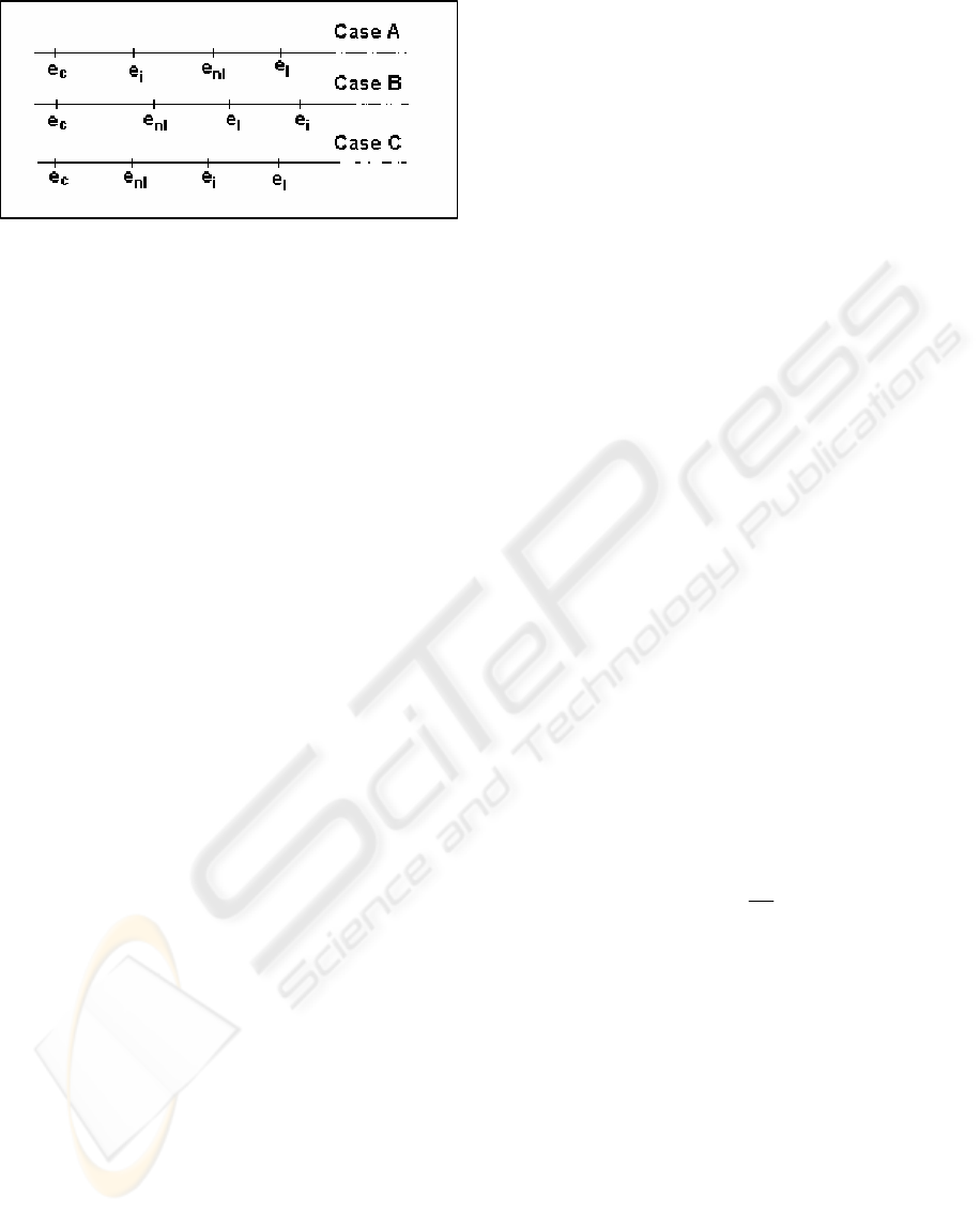
If the estimated parameters are arranged in a line
according to the geometrical error they generate,
several situations arise. The residual geometrical
error of the noise points with respect to themselves
is always cero e
c
=0. The geometrical error of the
ideal points q and p regarding to the noisy points q’
and p’ is always an unknown value called e
i
.
Additionally, there are geometrical errors with the
set of points generated with the parameters estimated
with linear methods and the parameters estimated
with non linear methods. These are called e
l
, e
nl
respectively. These errors are always known and
they will be bigger than the geometrical error cero
e
c
. Moreover, since the set of points resulting from
the non linear estimation has less geometrical error,
e
nl
will be always on the left side of e
l
. Now, the
essential question is, where is the unknown e
i
?. The
situation of this unknown, give us the efficiency of
the non linear estimation regarding the linear one. If
the exact parameters are those which generate a set
of points with a geometrical error e
i
, the goal is to
compute a set of parameters which generate a set of
points with a geometrical error close to the unknown
e
i
. Several situations showed in figure 1 arise.
In case A, better parameters will be always
obtained using non linear estimation. In this case,
since e
i
is on the left side of e
nl
, with the non linear
estimation better results will be obtained. In the case
B, since e
i
is on the right side of e
l
, with the non
linear finding worse camera parameters will be
computed. In the case C, the value of e
i
is between
e
nl
and e
l
. In this case, better results with the non
linear method will be obtained if e
nl
is closer to e
i
.
Since it is impossible to know the ideal points and
therefore e
i
, it is impossible to know if better results
will be obtained with the non linear method.
However, although it is impossible to know the
set of ideal points which give e
i
, it is possible to
know the noise level of the point’s coordinates. This
noise level gives the separation between e
i
and e
c
. If
the noise level is elevated, e
i
will be far from e
c
.
Otherwise, if the noise level is small, these values
will be closer. In the case of elevated level of noise,
the probability of obtaining a geometric error e
l
situated is case B is very high since e
i
and e
c
are
much separated. The set of parameters computed
with the non linear method generates points which
are closer of the noisy points. This means that the
estimation is worse although the residual
geometrical error is smaller. Therefore, with
elevated noise level it is more probably to obtain
worse results if the non linear method is used. From
the finding algorithm point of view, if the noise level
is high, the starting values of the parameters are far
from the ideal ones. This means that the finding
algorithm is unable to achieve the absolute minimum
and it is deviated to local one. This local minimum
gives worse values of the parameters although the
geometrical error is small. Otherwise if the noise
level is small, e
i
is closer to e
c
. Consequently, the
probability of e
l
is higher in the case A. In this case
the parameters computed with the non linear method
are better. The finding algorithm reduces the
geometrical error and it is closer to the ideal one.
Since the starting values of the parameters are close
to the ideal one, the finding algorithm stops close to
the absolute minimum.
The question now is how do we decide if use or
not non linear parameter estimation? The decision
should be based on the noise level of the
measurements of the points coordinates. Taking into
account that most of geometric computation
problems are χ
2
variables with r degrees of freedom,
where r depends on the application, it is possible to
know the noise level of the features coordinates.
This noise level ε
2
is computed knowing the residual
of the optimization. It is defined as
where I* is the residual of the optimization
(Kanatani 1995). It is necessary also to define the
limit of noise level for which the non linear
estimation deviates form the right solution. It should
be done testing each application. In this paper
camera calibration process has been tested.
In order to obtain better results, a new set of
point’s coordinates should be computed. If the
measured point’s coordinates are corrupted with
noise and the finding algorithm tries to satisfy it,
worse results will be obtained. Therefore, if a new
set of point’s coordinates with smaller level of noise
is satisfied, better results will be obtained.
Figure 1: Estimation methods arranged in a line, based on
their residual geometrical errors
r
I *
2
=
ε
WHEN SHOULD THE NON LINEAR CAMERA CALIBRATION BE CONSIDERED?
239
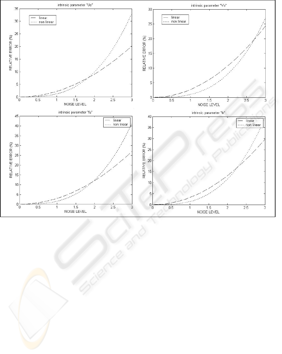
Figure 2: Relative error of estimated internal camera parameters
4 EXPERIMENTAL RESULTS
Both, simulated and real experiments have been
done to test the performance of the optimization
algorithms. First, calibration process with non linear
algorithms is tested with synthetic data to extract
conclusions about the influence of the noise level in
the computed parameters. Second, the overall
procedure is tested with real data provided with the
images o calibration template. This second series of
experiments demonstrates the validity of the overall
deduction.
4.1 Simulated experiments with
synthetic data
Several situations have been simulated in order to
extract some conclusion about non linear calibration
technique. A lot of different number of points of
interest has been used. This feature has no
significant effect on the estimated results from the
point of view of deviation of the non linear
parameters estimation. Finally, a set of 50 points in
the scene arranged into two planes has been used.
The camera is situated 1 m away form the Y axis,
with an angle of incidence of the camera optical axe
of 45 degrees with the X-Y plane. The starting
values of the parameters are computed with the
Direct Linear Transformation (DLT) algorithm
(Hartley 2000). A priori, no camera intrinsic
parameters are known. The non linear cost function
is not critical in order to test the deviation of the non
linear optimization. Similar results have been
computed. Depending on the used cost function, one
restriction or another is satisfied. Cost functions
which include the restriction of the camera
projection matrix have similar behaviour. The noise
level in the point’s coordinates is the only feature
which has a lot of effect in the estimated camera
parameters. The results are shown in figure 2. In this
experiment the noise level changes from 0 to 3
pixels in the image coordinate points and from 0 to 3
ICINCO 2005 - ROBOTICS AND AUTOMATION
240
mm in the 3D scene coordinate points. Steps of 0.1
have been taken. A set of points in the 3D scene
arranged into two planes is used and a camera ideal
model is generated with a set of intrinsic and
extrinsic parameters. This ideal model is represented
in a projection matrix which is used to calculate the
projections in the image of the 3D points in the
scene. Both sets of point’s coordinates (image and
scene) are corrupted with Gaussian noise. This
corrupted data is used to compute the camera
parameters, starting with the linear method and
finishing with the non linear one. This process is
done 100 times per step. After 100 times, the mean
of the estimated parameters with the linear method
and the non linear one are computed. Figure 2 shows
the result for each level of noise. It shows the
relative error for each value of the camera
parameters. The continuous line shows the linear
estimation and the dotted line is the non linear one.
In this case, non linear estimation is done without
any restriction included into the index. Results show
that, non linear calibration method can not improve
the results of the linear one, if the noise level is too
high. This result demonstrates the bad performance
of the non linear camera calibration method if the
noise level is high.
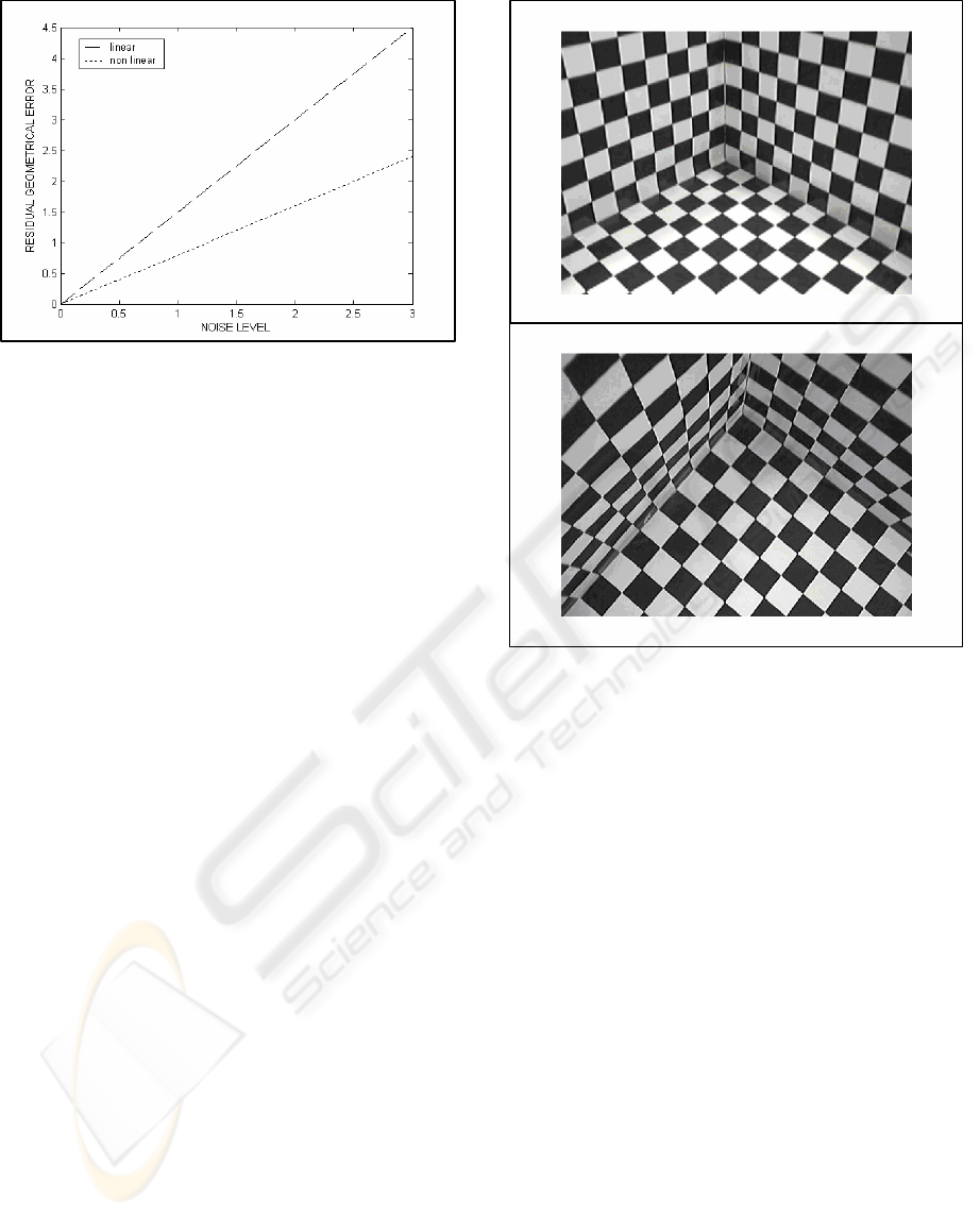
The term “to improve the results” should not be
interpreted as to reduce the geometrical error. It is
true that the non linear camera calibration method
reduces the geometrical error but from a practical
point of view, this method computes worse values of
the absolute camera model parameters. Figure 3
shows the residual optimization using linear and non
linear optimization method. It is clear that the non
linear optimization method reduces the geometrical
error a lot, but when the noise level is high, this
reduction does not improve the absolute values of
the parameters.
Seeing the figures, the noise level from which the
non linear optimization method computes worst
results is about 2.1.
4.2 Experiments with real images
From the point of view of calibration of a real
camera, images from different positions are taken of
a calibration template. Calibration images are shown
in figure 4. Images from different positions are taken
to detect the coordinates of the calibration points
with different accuracy. Then, the noise level of
points coordinates changes. With these points, the
calibration process has been carried out in the same
way as in the simulation stage. Camera has been
calibrated 100 times in order to extract mean values.
Smaller residual optimization has been computed
with non linear optimization techniques. Also,
different parameters have been computed with each
method. Since the real values of camera parameters
are not known it is impossible to decide which
calibration is better. However, the noise level of the
points coordinates computed with the χ
2
test can
help us to decide. In this case noise level about 2 has
been computed with images 2 and 3 as is shown in
Figure 3: Residual geometrical error with linear and non
linear method
Figure 4: Images of the calibration template
WHEN SHOULD THE NON LINEAR CAMERA CALIBRATION BE CONSIDERED?
241

table 1. Taking into account the simulated results, no
linear optimization method should be discarded or
better detection of the points coordinates in the
image should be done. In this case, better calibration
stage should be used.
Table 1: Results of experiments with real data
Residual optimization
Lineal Non linear
Noise
level ε
2
Image 1 2.901 1.588 1.224
Image 2 5.687 1.026 2.345
These results can be extrapolated to any
parameter estimation process. It is necessary to take
into account the noise level of the input data before
using non linear optimization techniques.
5 CONCLUSIONS
For parameters estimation, the non linear
optimization method can be useful if the noise level
of the input data is not very high. If the noise level is
too high, the non linear optimization technique
computes worst absolute results. The algorithm
converges to a local minimum which improve the
geometrical error but not absolute values of the
parameters, even using the Levenberg-Marquardt
finding algorithm. Non linear optimization
minimizes a cost function with a lot of degrees of
freedom and it can diverge to false results if the
noise level is very high. In these cases linear
parameter estimation methods are faster and achieve
better results. In order to improve parameter
estimation process using non linear techniques, low
noise input data should be used.
REFERENCES
F. Dornaika and C. Garcia, 1997, Robust camera
calibration using 2D to 3D feature correspondences,
International Symposium SPIE, San Diego.
O. Faugeras, 1993, Three dimensional computer vision,
The MIT Press, Massachusetts.
R. Hartley and A. Zisserman, 2000, Multiple View
geometry in computer vision, Cambridge, United
Kingdom
J. Heikkilä and O. Silven, 1997, A four step camera
calibration procedure with implicit image correction,
IEEE Computer Society Conference on Computer
Vision and Pattern Recognition, San Juan, Puerto Rico.
K. Kanatani, 1995, Statistical optimization for geometric
computation, Springer.
W. Press, B. Flannery, S. Teukolsky, W. Vetterling, 1988,
Numerical recipes in C, Cambridge, United Kingdom.
ICINCO 2005 - ROBOTICS AND AUTOMATION
242
