KNOWLEDGE REPRESENTATION APPROACH TO CLOSED LOOP
CONTROL SYSTEM - A TANK SYSTEM CASE-STUDY
Lu
´
ıs Rato, Irene Pimenta Rodrigues, Rui Gomes
Universidade de
´
Evora
R. Rom
˜
ao Ramalho, 59, 7000-671
´
Evora
Keywords:
Control, declarative programming, knowledge representation, constraints.
Abstract:
Control engineering problems are dealt within a plethora of methods and approaches depending on the a priori
knowledge, the description of the process to control, and the main control goal. Classical control theory is
mainly based on properties of numerical models. This paper presents an approach that applies to a class of
processes described by numerical and logical relations using inference and a knowledge base system. To attain
this goal an ontology for control systems is constructed. The work presented in this paper is based in a three
tank system benchmark.
1 INTRODUCTION
The knowledge representation as a major impact on
the performance of intelligent systems (Messina et al.,
2001) and the relevance of this fact increases with the
complexity of systems we are dealing with. Thus,
considering the diversity and the potential complex-
ity of control engineering problems one must consider
that control systems are a natural candidate to apply
knowledge bases and inference systems.
Most applications of artificial intelligence algo-
rithms to control problems amount to softcomput-
ing techniques and supervision tasks (Shadbolt et al.,
1989). Nevertheless, the concern on modelization
from the control engineering community has pro-
duced some work on component oriented model lan-
guage as in the Modelica language (Elmqvist et al.,
2001) or CSML (Zagar et al., 2001). In this work we
aim to describe, infer the behaviour, and infer control
actions in a integrated way through a Prolog imple-
mentation using finite domain constraints (Diaz and
Codognet, 2000; Sterling and Shapiro, 1997).
Although the importance of knowledge represen-
tation is recognised and Prolog is used to express
declarative rules about controller properties in (Shad-
bolt et al., 1989), the inference system remains lim-
ited to supervision tasks. This work presents a more
integrated approach from process description to con-
trol tasks and aims to be as general as possible.
The scope broadening of such approach will be at-
tained with a penalty in efficiency when compared to
the very powerfull classical linear system tools. Thus,
in order to illustrate the potential of such approach a
non linear, multi-input multi-output (MIMO) system
is chosen as a test-case. For such systems the power-
full mathematical tools are restricted to very particu-
lar cases. Another possible approach is to combine in-
teger programming with real constraint optimisation
(Bemporad and Morari, 1999). Nevertheless, such
tools do not have a programming framework to sup-
port them as powerful as logic programming has. The
test-case used in this work, a three-tank system, has
been used as a very flexible benchmark system for re-
configurable control techniques (Lunze et al., 2001).
This paper is organised as follows. An introduction
is made in section 1. Section 2 presents the knowl-
edge based control system build around the three tank
system test-case. The model is validated by simula-
tion in Section 3. Section 4 presents the queries that
solve the proposed control problems. Some conclu-
sion are addressed in Section 5.
2 KNOWLEDGE BASED
CONTROL SYSTEM
In this section a knowledge based control system is
build around the three tank system test-case. Though
the knowledge based system presented here does not
113
Rato L., Pimenta Rodrigues I. and Gomes R. (2005).
KNOWLEDGE REPRESENTATION APPROACH TO CLOSED LOOP CONTROL SYSTEM - A TANK SYSTEM CASE-STUDY.
In Proceedings of the Second International Conference on Informatics in Control, Automation and Robotics, pages 113-118
DOI: 10.5220/0001186301130118
Copyright
c
 SciTePress

aim to a general purpose solution to process mod-
elling and control it presents solutions that can be eas-
ily extended to other processes and control problems.
Some of the control problems that we aim to ad-
dress are: estimation, fault detection and isolation,
control actuation, and controller optimisation. These
control problems can be define in a declarative way
according to:
• Estimation - given a series of observations of the
process which are the possible internal states at in-
stant t.
• Fault detection and diagnosis - given a series of ob-
servations of the process which are the admissible
models or model variations.
• Control actuation - given a series of observations
and a control goal (control reference) which should
be the actuation on the process such that the goal is
attained at an instant t.
• Controller optimisation - given process and con-
troller models which are the controller parameter-
ers such that the closed loop system is optimal ac-
cording to a criteria (penalty function).
These set of classical control problems may be de-
fined with constraints such as internal state variables,
solution space, and time constraints. This fact sug-
gests the use of a constraint oriented programing tool.
2.1 Linear dynamical system
In order to illustrate the potential of the proposed
approach consider a discrete-time linear dynamical
system to be represented in logic programming with
constraints. Discrete-time is considered since the
GnuProlog constraint system applies only to integer
domain.
x(t +1)=Ax(t)+Bu(t) (1)
y(t)=Cx(t)+Du(t) (2)
where x(t) is the state; u(t) is the input; y(t) is the
output and A, B, C, D are matrices which parame-
terise the linear system. The following problems will
be considered:
• Simulation - given parameters A,B,C,D, the input
u(t) and initial conditions x(0) what is the state x
or output y at a certain instant t
• Input definition - given parameters A,B,C,D, the
desired output y at time t (with an error marginδ),
initial conditions x(0) what are the possible inputs
u(t) (with some constaints, e.g. constant input).
• Parameterisation - given parameters A,B,C,D, par-
tially defined, the input u(t) and initial conditions
x(0) what should be the parameters such that the
output y is the desired one at time t (with an error
margin
δ)
Prolog Implementation
Two predicates are defined to implement the state and
output equations. The predicate ”state” defines the
state x(t +1)recursively
state(XT1,T1) :- T1 #= T+1, state(XT,T),
input(UT,T),
XT1 #= A
*
XT+B
*
UT.
and the predicate ”output” defines the output y(t)
output(YT,T) :- state(XT,T), input(UT,T),
YT #= C
*
XT + D
*
UT
where A, B, C, D stands for the linear system para-
meters; XT is the state x(t), XT is the input u(t) and
YT is output YT. It should be noted that, in general,
the operators ”*” and ”+” represent the matrix product
and sum, and the variables XT, YT and UT are vec-
tors with compatible dimensions. Furthermore, since
GNU-Prolog constraint solver operates only on inte-
ger positive values, operators ”*” and ”+” and number
representation must be such that positive and negative
limited precision real values are represented through
integer positive values.
To attain this goal negative integer are represented
using tens complements. This is a particular case of
a modular arithmetic (modulo a ten’s power) (Knuth,
1997), just as two’s complements in computer arith-
metic. In order to represent decimal part, variables
are scaled by a constant 10
n
.
Initial contitions may be introduced through a fact
such as
state(0,0).
which stands for x(0) = 0 in a first order system.
Consider the simulation problem. Given zero initial
conditions, and constant input u(t)=1, the value
XT unifies to 1 for any time T .
input(1,_).
the following query defines the output at instant 100.
output(YT,100).
The second proposed problem is input definition.
Given a desired output y = yout with a certain toler-
ance tol, at time t = 100 what should be the input, if
it is constant.
% constant input
input(T1,U) :- T1 #= T+1, input(T,U)
the query could be defined as
input(0,U), output(Y,100),
Y #< yout+tol , y #> yout-tol.
where yout and tol are the desired output value and
tolerance; and U is the variable that unifies with a so-
lution.
ICINCO 2005 - INTELLIGENT CONTROL SYSTEMS AND OPTIMIZATION
114

2.2 Tank System case-study
The three tank system, in figure 1, is a rich benchmark
system due to its nonlinear behaviour, actuators and
sensors which can be continuous as well as on-off,
and redundancy which allows to test reconfigurable
control strategies(Rato and Lemos, 1999). Control re-
configuration is a control problem usually tackled by
non classical control tools, thus a good candidate to il-
lustrate the potential of a knowledge based approach.
Tank2
Source1
Source2
Valv13
Valv32
ValvL
Valv2
Valv1
SensorLevel3
SensorLevel1
Controller PI1
Tank1
ControllerON−OFF1
Tank3
PI
controller
ON−OFF
controller
Figure 1: Tree tank system
The mathematical model of tank systems are repre-
sented by the following differential equation for each
tank,
˙
h(t)=
N

i=1
Q
i
(t)
A
T
(3)
where A
T
is the area of the tank base’s, N is the
number of inputs/outputs, and Q
i
is the inflow in each
tank’s input/output. External sources are manipulated
variables.
Q
i
(t)=u(t) (4)
and whenever there is a pipe at height h
p
(only con-
stant section horizontal pipes are considered in this
work) between two tanks the inflow is defined by:
if h>h
p
and h

>h
p
Q
i
(t)=a
Z
Ssgn(h

− h)

2g|h

− h| (5)
if h>h
p
and h

<h
p
Q
i
(t)=a
Z
Ssgn(h

− h
p
)

2g|h

− h
p
| (6)
if h<h
p
and h

>h
p
Q
i
(t)=a
Z
Ssgn(h − h
p
)

2g|h − h
p
| (7)
if h<h
p
and h

<h
p
Q
i
(t)=0 (8)
where h is the level of the tank being modelled; h

is
the level of another tank connected at height h
p
.
The three tank system is composed by three tanks
6m high, with a section surface S =3.610
−5
m
2
,
Figure 2: Catalog of individuals
Figure 3: Model representation
with 2 pipes connecting the central tank to each one
of the other two tanks - one at h =0and an-
other at h =0.3 m - each pipe with section surface
A =0.0154 m
2
has a valve and there are two pumps
that put water into tanks 1 and 2. Maximum flow
for each pump is Q
max
=0.110
−3
ms
−1
Constant
a
z
is assumed unitary. The level of the tanks can be
controlled using the flow from the pumps as well as
through the valves.
A complete model description may be found in
(Lunze et al., 2001). The continuous time model
is obtained discretizing the continuous model using
Euler’s method (
˚
Astr
¨
om and Wittenmark, 1997).
2.3 Three tanks representation as a
Finite Domain Constraint
Satisfaction Problem
To represent the three tanks systems as a constraint
satisfaction problem in Prolog we had to build an on-
tology in order to represent the system entities and its
proprieties.
In figure 2 we present a excerpt of the defined con-
ceptual graph for representing our domain ontology
(three tanks problem). In figure 4 we present the de-
scription of an example according to the ontology de-
fined in figure 2.
In Prolog with finite domain constraints our enti-
ties may be represented by: names, constants values,
KNOWLEDGE REPRESENTATION APPROACH TO CLOSED LOOP CONTROL SYSTEM - A TANK SYSTEM
CASE-STUDY
115

tank(t1,6.0,1.54).
hasHole(t1,hl1).
hasHole(t1,hl2).
hasHole(t1,hl3).
hole(hl1,3.6E-3,3.0).
hole(hl2,3.6E-3,0.0).
hole(hl3,3.6E-3,0.0).
links(hl1,p1).
links(hl2,p2).
links(hl3,p3).
source(s1,0.1).
on(s11,t1).
Figure 4: Representation of a three thanks configuration
variables or constraint variables. Proprieties are rep-
resented by predicates that relate one or more entities.
In this paper we will detail the representation of the
proprieties:
• Tank level height
In our ontology tanks have the propriety of having
a level hight at a time instant, this is represented
by the 3 arguments predicate h where the first ar-
gument represents the tank name, the second one is
a constraint variable that represents the tank hight
and the third one is a constraint variable that repre-
sents a time instant
Example: h(t1,HT,T), represents that tank t1 has
height HT at the time instant T.
The height value, as we can see from equation ??,
at a time instant depends on the flow of the pipes or
sources connected to the tank.
• Pipes and sources flow.
Pipes are connected to tanks and have the propertie
of having a flow at a time instant. The predicate to
represent the flow of a pipe or a source is a 3 argu-
ments predicate q where the first argument repre-
sents the pipe or source name, the second one is a
constraint variable that represents the pipe flow and
the third one is a constraint variable that represents
a time instant.
Example:
q(p1,QT,T), represents that pipe p1 has flow QT at
the time instant T.
q(s1,QT,T), represents that source s1 has flow QT
at the time instant T.
In order to model the behaviour of three tanks rep-
resented in figure 1 we had to define a set of rules such
has the following ones:
• rule to model Tank t1 level height
h(t1,HT,T):- T1#= T-1, h(t1,HT1,T1),
q(s1,Fs1,T1),
q(hl1,Fhl1,T1),
q(hl2,Fhl2,T1),
area(t1,A),
HT #= HT1 + (Fs1+Fhl1+Fhl2) /|/ A.
The operator //— represents the integer division
between integer represented in ten-complement.
Flow and height values are represented in ten-
complement since flows in pipes may be positive
or negative.
• rule to model Tank1 t1 initial conditions
Supposing that the initial conditions where that
thank 1 has a level less then 10until 5 seconds. The
following rule represents this initial conditions.
h(t1,H,T):- H#<10,T#<5.
• rule to model flow in source s1
The following rule states that source s1 has a flow
of 20 from t=0 until t=10.
q(s1,FT,T):- FT#=20, T#>=0,T#=10.
• rule to model flow in pipe p1.
This rule will be obtain from the general equations
presented in the previous subsection taking into ac-
count that pipe p1 connects tank t1 and tank t2.
For instance the translation of the rule:
if h>h
p
and h

>h
p
Q
i
(t)=a
Z
Ssgn(h

− h)

2g|h

− h| (9)
q(p1,FT,T):- T1 #= T-1,
h(t1,HT1,T1),
h(t2,HT2,T1),
height(p1,H),
HT1#>H, HT2#>H,
HD#= HT1-HT,
module(HD,HDM),
FT1
*
FT1 #= 2
*
10
*
HDM,
signal(HD,FT1,FT).
3 CONTROL AND DIAGNOSIS
QUERIES
In this section we present some examples in order to
illustrate the results of our modulation of the three
tanks using logic programing with finite domain con-
straints.
ICINCO 2005 - INTELLIGENT CONTROL SYSTEMS AND OPTIMIZATION
116

3.1 Model validation
The generated declarative model of the tank system
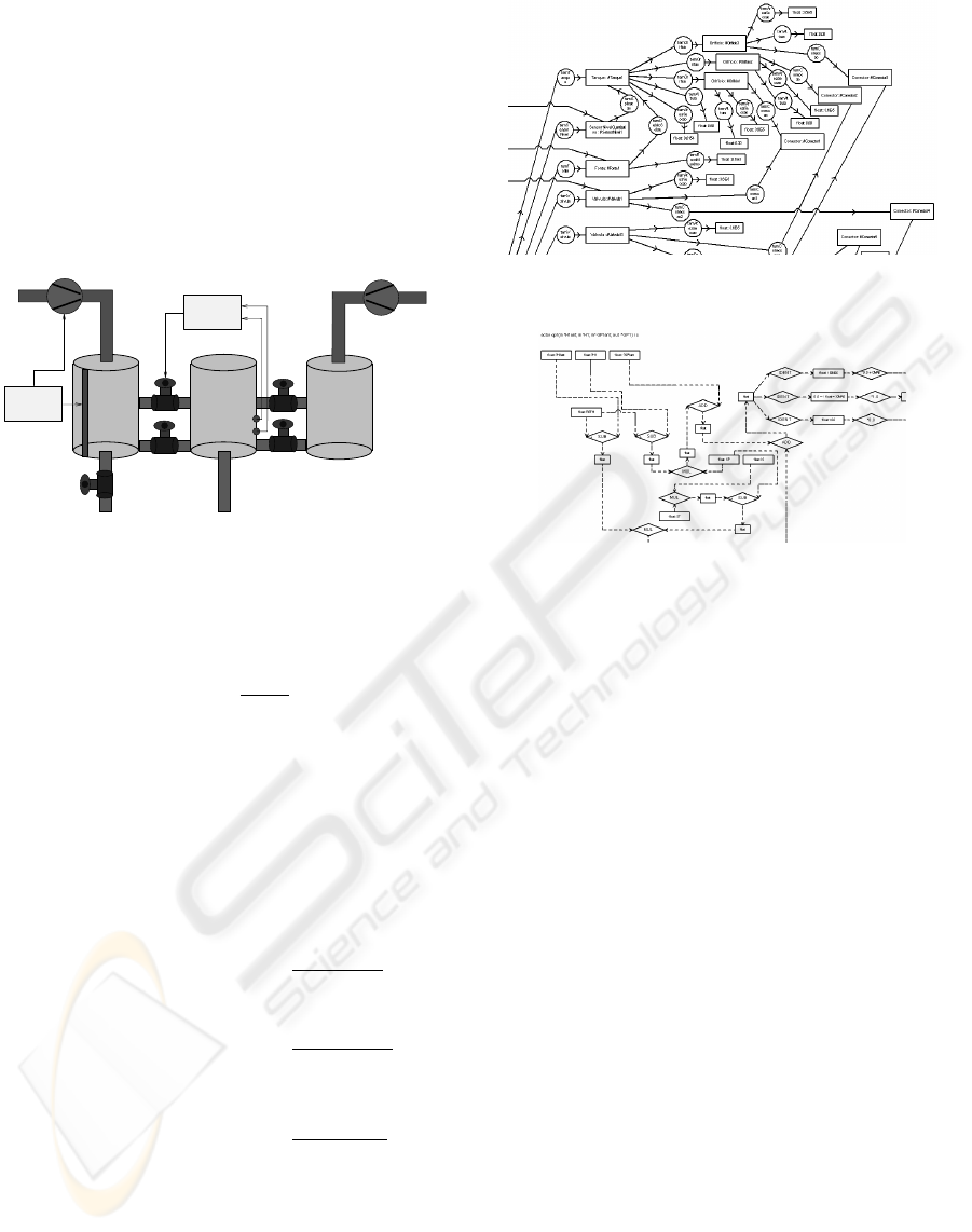
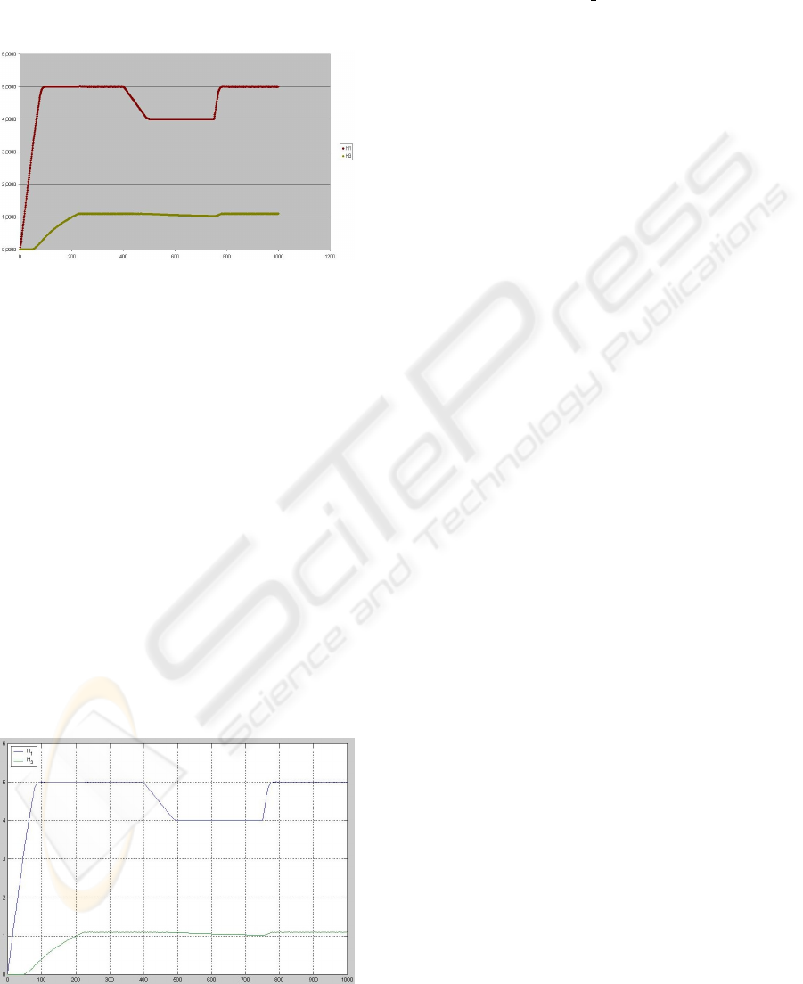
is validated comparing simulation results in figure 5
with results from a MATLAB implemented model ac-
cording to (Lunze et al., 2001), in figure 6
Figure 5: Three tank system simulation - GNU-Prolog
The results of the generated declarative model im-
plemented in PROLOG with finite domain constraints
are according to those from the MATLAB simulation.
3.2 Example 1 - A diagnosis problem
Consider the tank system and admit that a leakage
may occur. This fault is simulated by opening of
valve 1L which is in the bottom of tank 1, at instant
t = 160. One may wish to find in which instants such
a fault may occur considering the observations. This
amounts to a diagnosis problem.
The following constraints were considered: the
fault occurs in the interval 150s<t<175s;
the model is admissible if the simulated tank level
h
s
imul and the observations are such that |h
simul
−
h
obs
| < 10mm. The query is,
| ?- findall(T,(T#<300,
h(t1,HT,T),
Figure 6: Three tank system simulation - MATLAB
h_obs(t1,HobsT,T),
(HT-HobsT)#<10) ,LS).
LS = [159,160,161]
Where the predicate h obs is in the database de-
fined for all relevant time instants, 0 to 300.
If the solutions are ordered by decreasing error
then,
| ?- setof(DT-T,(T#<300,
h(t1,HT,T),
h_obs(t1,HobsT,T),
DT#= HT-HobsT,
DT#<10),LSO).
LSO = [0-160,7465-161,8099-159]
the instant t = 160 is the most likely to be the correct
answer. It should be noticed that in this simulations
there is not addition of noise on sensor signals so, ex-
act answers are found.
3.3 Example 2 - control problem
with constraints
Consider the goal is to have the tank level at 205mm
at instant t =60s. We should define the input flow Q
(from a pump) considering this flow to be constant
in the interval 0s<t<60s with the constraint
75000mm/s < Q < 80000mm/s.
This constraints could be stated by the following
rules:
q(s1,FT,T):- FT#<80000, FT#>75000, T#<60,T#>60.
h(t1,205,T):- T#=60,!.
This amounts to a control problem with constraints,
whose solution is obtained by the query,
| ?- findall(FT,q(s1,FT,60),LS).
LS = [75844,75845,75846,75847,75848,
75849,75872,75873,75874,75875]
where the predicate h(t1,HT,T),T#=60cal-
culates the tank level at t =60s. This results depends
on the initial conditions of the tank system. Thus, one
of those solutions can be applied in a received strat-
egy. Which means that after the solution is obtained
and applied, new observations are made and a new
solution is calculated.
3.4 Example 3 - calculating optimal
gains
Consider the tank water level in closed-loop con-
trolled by a fixed structure controller such as a PI
controller. We want to determine the controller para-
meters under the following constraints: the controller
gains (proportional gain k
p
and integral gain k
i
) are
in the intervals 1 <k
i
< 10 and 10 <k
p
< 100; the
tracking error (the difference between the goal and the
actual level) is bounded to 5mm ref − h| =< 5mm;
KNOWLEDGE REPRESENTATION APPROACH TO CLOSED LOOP CONTROL SYSTEM - A TANK SYSTEM
CASE-STUDY
117

and there is no overflow in the tank h<600mm
within the following time interval 25s<t<100s.
which is solved by the following query, whose set of
solutions is over 200.
| ?- findall((KP,KI),sim(KP,KI,_),LS).
LS = [(25,2),(26,2),(27,2),(30,3),...]
where sim(KP,KI,ERR TOTAL) is a predicate
that calculates the tracking error of the closed loop
system with gains K
i
and K
p
.
An optimal parameterisation is obtained with a in-
creasing error ordered list
| ?- setof(ET-(KP,KI),sim(KP,KI,ET),LSO).
LSO = [3330-(75,10),3337-(74,10),....]
resulting in the optimal gains K
i
=10and K
p
=75.
4 CONCLUSIONS AND FUTURE
WORK
A declarative approach to control problems that ap-
plies to a class of processes described by numerical
and logical relations using inference and a knowledge
base system as been presented. Logic programming
with constraints has been applied. The followed ap-
proach makes possible not only to represent the con-
trol system in declarative way but also to query the
knowledge base system using the same declarative
language. The complete system is described using
the same description language no matter we are deal-
ing with logical or numerical variables. A further step
in the research will be to explore constraint logic pro-
gramming using other solvers that cope with real vari-
ables (positive or negative) possibly using mixed inte-
ger quadratic optimisation and compare the precision
gains versus the computational complexity increase.
Another problem that should be carefully analysed,
in the presence of quantisation, is the propagation of
quantisation error across the inference process.
REFERENCES
˚
Astr
¨
om, K. and Wittenmark, B. (1997). Computer Con-
trolled Systems. Prentice-Hall.
Bemporad, A. and Morari, M. (1999). Control of systems
integrating logic, dynamics, and constraints. Automat-
ica.
Diaz, D. and Codognet, P. (2000). The gnu prolog sys-
tem and its implementation. In ACM Symposium on
Applied Computing-SAC, Villa Olmo, Como, Italy.
ACM.
Elmqvist, H., Mattson, S., Otter, M., and Astrm, K. (2001).
Modeling complex systems. In Astrm, K., Albertos,
P., Isidori, A., Schaufelberger, W., and Sanz, R., edi-
tors, Control of Complex Systems, chapter 2. Springer.
Knuth, D. (1997). The Art of Computer Programming -
Seminumerical Algorithms. Addison-Wesley.
Lunze, J., Askari-Marnani, J., Cela, A., Rato, L., Lemos,
J., and Staroswiecki, M. (2001). Three-tank control
reconfiguration. In Astrm, K., Albertos, P., Isidori,
A., Schaufelberger, W., and Sanz, R., editors, Control
of Complex Systems, chapter 2. Springer.
Messina, E. R., Evans, J. M., and Albus, J. S. (2001). Eval-
uating knowledge and representation for intelligent
control. In 2001 PerMIS Workshop, Mexico.
Rato, L. and Lemos, J. M. (1999). Multimodel based fault
tolerant control of the 3-tank system. In Proceedings
of European Control Conference ECC99, Karlsruhe,
Germany.
Shadbolt, N. R., Robinson, B. D., and Stobart, R. K. (1989).
knowledge represebtation for closed loop control. In
SIGART: ACM Special interest group on AI.ACM
Press.
Sterling, L. and Shapiro, E. (1997). The Art of Prolog. MIT
Press.
Zagar, K., Plesko, M., G.Tkacik, and Vodovnnik, A.
(2001). The control system modelling language. In
ICALEPCS-2002, San Jose CA.
ICINCO 2005 - INTELLIGENT CONTROL SYSTEMS AND OPTIMIZATION
118