
PIECEWISE AFFINE SYSTEMS CONTROLLABILITY AND
HYBRID OPTIMAL CONTROL
Aude Rondepierre
Laboratoire de Mod
´
elisation et Calcul
50 av. des Math
´
ematiques - 38041 Grenoble, France
Keywords:
Piecewise affine hybrid systems, polyhedral sets, controllability, optimal control synthesis, algorithms.
Abstract:
We consider a particular class of hybrid systems, defined by a piecewise affine dynamic over non-overlapping
regions of the state space. We want to control their behaviors so that it reaches a target by minimizing a given
cost. We provide a new numerical algorithm under-approximating the controllable domain under the given
hybrid dynamic. Given an optimal sequence of states of the hybrid automaton, we are then able to traverse the
automaton till the target, locally insuring optimality.
1 INTRODUCTION
Aerospace engineering, automatics and other indus-
tries provide a lot of optimization problems, which
can be described by optimal control formulations:
change of satellites orbits, flight planning, motion co-
ordination (Fierro et al., 2001; Pesch, 1994). Since the
years 1950-1970, the optimal control theory has been
extensively developed and provides us with powerful
results like dynamic programming (Bellman, 1957)
or the maximum principle (Pontryagin et al., 1974).
However resolutions are mainly numerical.
Now, in “real-life”, optimal control problems are
fully nonlinear. There are today two main classes
of numerical methods: the first one uses a discrete
version of the dynamical principle (Bertsekas, 1984;
Bardi and Capuzzo-Dolcetta, 1997). But those algo-
rithms are very expensive in high dimension. The
second is based on the Pontryagin Maximum Princi-
ple (Pontryagin et al., 1974), (Bryson and Ho, 1975),
which provides a pseudo-Hamiltonian formulation of
optimal control problems. However, the main diffi-
culty is actually the synthesis of optimal feedback,
even not solved for linear systems, except in some
very special cases as time-optimal problems (Bryson
and Ho, 1975; Pinch, 1993; Pesch, 1994).
In this paper, we consider a particular class of hy-
brid systems, defined by a piecewise affine dynamic
over non-overlapping regions of the state space:
˙
X(t) = A
q
X(t)+B
q
u(t)+c
q
, for X(t) ∈ D
q
(1)
We present a hybrid algorithm controlling the system
(1) from an initial state X
0
at time t = 0 to a final
state X
f
= 0 at an unspecified time t
f
. To reach
this state, we allow the admissible control functions
u to take values in a convex and compact polyhedral
set U
m
of R
m
, in such a way that: J(X, u(.)) =
R
t
f
0
l(X(t), u(t))dt is minimized.
Piecewise affine models has become a relevant and
powerful tool in the approximation of general smooth
nonlinear systems (Johansson, 1999). They usually
manage to capture many features of general physical
systems, and enable a tractable mathematical analy-
sis. Where usual numerical methods suffers from
the curse of the dimension (and with the expansion
of aerospace, today algorithms in the control theory
have to deal with dimension 6 or 7), the analytical
approach by piecewise affine models must allow to
improve approximations (Girard, 2004): the level of
details allows to reach a compromise between quanti-
tative quality of the approximation and the computa-
tional time. Such studies has already be done e.g. for
biological systems, where simplifications in relation
to real data and in regard of simulations are possible,
see (Dumas and Rondepierre, 2003).
Here, we provide a full implementation for the analy-
sis of polyhedral piecewise affine control systems
in every dimension. In particular, we develop a
new efficient numerical method to compute an under-
approximation of the controllable domain. We also
propose some promising directions towards generic
algorithms for solving piecewise affine optimal con-
trol problems.
The paper is organized as follows. In section 2, we de-
fine hybrid systems and formulate the hybrid optimal
control problem. In section 3, we provide a numeri-
cal controllability analysis and then, in section 4, an
294
Rondepierre A. (2005).
PIECEWISE AFFINE SYSTEMS CONTROLLABILITY AND HYBRID OPTIMAL CONTROL.
In Proceedings of the Second International Conference on Informatics in Control, Automation and Robotics - Signal Processing, Systems Modeling and
Control, pages 294-299
DOI: 10.5220/0001185802940299
Copyright
c
SciTePress

algorithmic resolution of the hybrid optimal control
problem. Some examples are presented in section 5.
2 HYBRID OPTIMAL CONTROL
PROBLEM
Let us start defining our hybrid problem. The con-
trol domain U
m
is a polytope in R
m
, defined as the
convex hull of a finite number of points: U
m
=
Conv(s
1
, . . . , s
p
), such that: 0 ∈ U
m
. The points
s
i
are assumed to be the vertices of U
m
.
Let (D
q
)
q
be a polyhedral partition of the state
space R
n
. We thus introduce the hybrid automaton
H = (Q, D, E, F, G, R) defined as follows:
1. Q the countable set of indices of the simplexes D
q
.
2. D = {D
q
/ q ∈ Q} the collection of domains over
the state space: ∀q ∈ Q, D
q
is a polyhedron of R
n
∀(q, q
′
) ∈ Q
2
, [int(D
q
)∩int(D
q
′
) 6= ∅ ⇒ D
q
= D
q
′
]
3. E = {(q, q
′
) ∈ Q × Q/ ∂D
q
∩ ∂D
q
′
6= ∅} the
transition set.
4. F = {f
q
/ q ∈ Q} the collection of affine field
vectors:
f
q
: D
q
× U
m
→ R
n
(X, u) → A
q
X + B
q
u + c
q
such that: [ 0 ∈ D
q
⇒ c
q
= 0 ].
5. G = {G
e
/ e ∈ E} the collection of the guards:
∀e = (q, q
′
) ∈ E, G
e
= ∂D
q
∩ ∂D
q
′
6. R = {R
e
/e ∈ E} the collection of Reset func-
tions: ∀e = (q, q
′
) ∈ E, ∀x ∈ G
e
, R
e
(x) = {x}
(Here, we do not need to reinitialize the continuous
variable x, since the D
q
are adjacent).
Remark 1 The assumption [ 0 ∈ D
q
⇒ c
q
= 0 ]
ensures that the target 0 is an equilibrium point of
our hybrid dynamic for u = 0.
From now on, the hybrid automaton H is assumed not
Zeno
1
.
In this paper, we focus on optimal control problems
(P
H
) associated to the hybrid automaton H ; we con-
sider the hybrid dynamic induced by H:
˙
X(t) = A
q
X(t)+B
q
u(t)+c
q
, for X(t) ∈ D
q
(2)
and want to control (2) from an initial state X
0
to a
target X
f
= 0 at an unspecified time t
f
. To reach this
state, we allow the admissible control functions u to
take values in the polytope U
m
, in such a way that:
J(X, u(.)) =
R
t
f
0
l(X(t), u(t))dt is minimized.
1
Zeno executions correspond to an infinite number of
switch in a finite time. That often involves problems in the
simulation of hybrid system. Indeed the transition times
come closer and closer and in simulations, we can not dif-
ferentiate them any more (see (Girard, 2004; Zhang et al.,
2001)).
3 HYBRID SYSTEM
CONTROLLABILITY
In this section, we want to compute the set of con-
trollable points in R
n
, i.e. the set of initial points
for which the hybrid problem (P
H
) admits a solution.
The idea is, by time reversal, to come down to the
computation of the attainable set from 0 and to guar-
antee the controllability of given initial points.
In (Dumas and Rondepierre, 2005, §3.1), an algo-
rithm is proposed to compute an under-approximation
in time T of the controllable set for linear systems
without state constraints. In this paper, we propose
an extension of this algorithm to piecewise affine sys-
tems. First we present our under-approximating al-
gorithm over one given cell of the space state. This
enables us then to build an under-approximation of
the controllable set over a path of cells.
3.1 Under-Approximation of the
Controllable set in a given cell
Let q be a discrete mode satisfying: 0 ∈ D
q
. We
want to compute an under-approximation of the con-
trollable set inside the cell D
q
⊂ R
n
under the control
constraints: u ∈ U
m
= Conv(s
1
, . . . , s
p
).
Definition 1 (Controllable set in D
q
when 0 ∈ D
q
)
X ∈ D
q
is controllable iff there exist T ≥ 0 and
u : [0, T ] → U
m
admissible, such that:
i. X = −
R
T
0
e
−A
q
ω
[B
q
u(ω) + c
q
]dω
ii. ∀t ∈ [0, T ], −
t
0
e
−A
q
ω
[B
q
u(ω) + c
q
]dω ∈ D
q
In the next, X
q
[0, s
i
](.) denotes the trajectory accord-
ing to u = s
i
that goes through 0 ; then, by time rever-
sal, X
q ,i
denotes the first intersection of X
q
[0, s
i
](.)
with ∂D
q
. Let F
q ,i
be the encountered face:
X
q ,i
= X[0, s
i
](T
i
) ∈ F
q ,i
where: T
i
= sup{t < 0/ X[0, s
i
](t) ∈ ∂D
q
} as
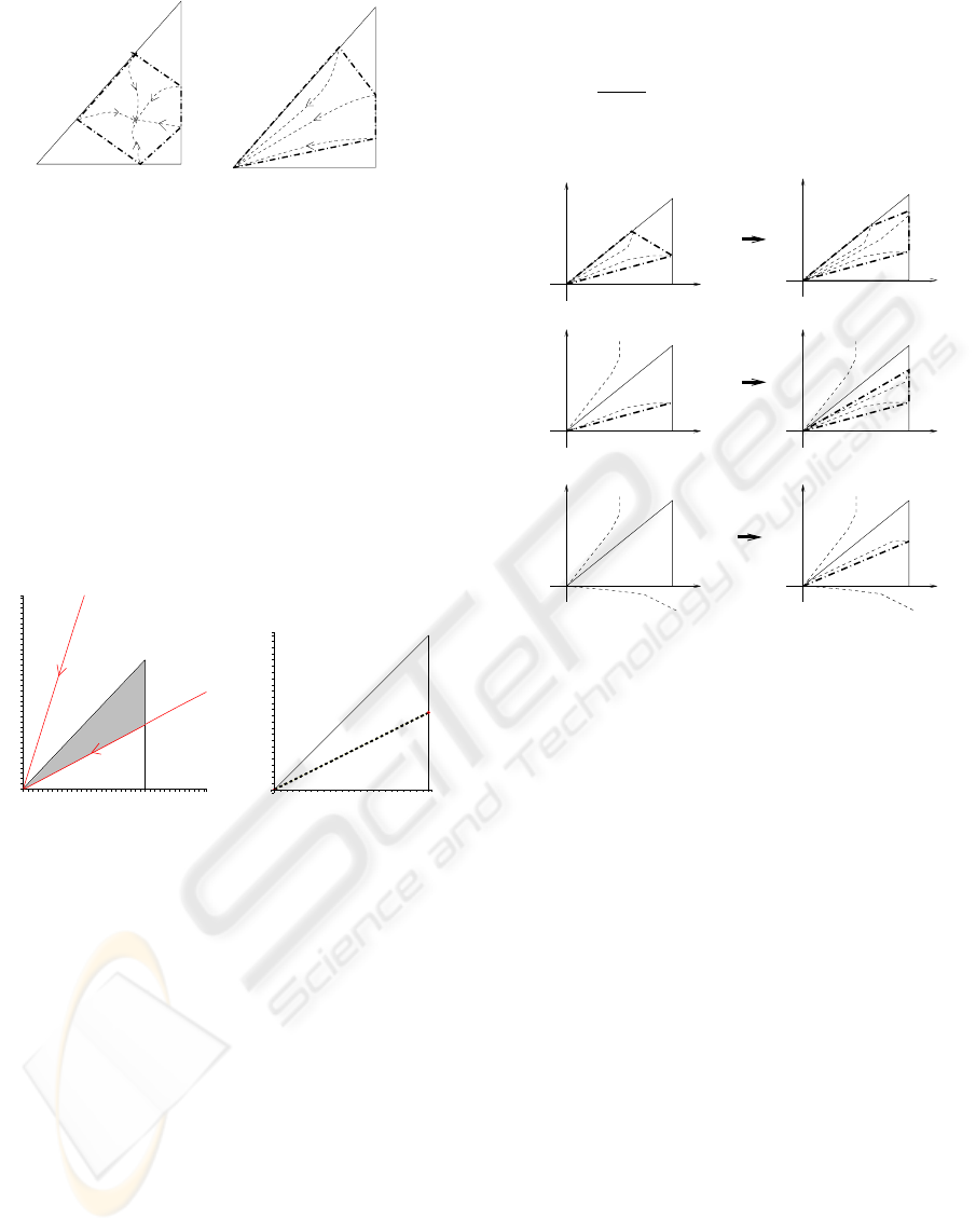
shown on figure 1.
Notation 1 (X
q ,i
, F
q ,i
) := OutCell(q, 0, s
i
)
By convention, when X
q
[0, s
i
](.) goes out of D
q
, we
state: (X
q ,i
, F
q ,i
) = (∅, ∅).
By linearity of the hybrid dynamic in the mode q, the
controllable domain in D
q
is convex and (Dumas and
Rondepierre, 2005, Proposition 3) can be applied in
our context:
Proposition 1 Conv(X
q ,1
, . . . , X
q ,k
) is an under-
approximation of the controllable set in D
q
.
However the quality of the resulting under-
approximation is very poor, especially when
most of trajectories do not evolve inside D
q
.
PIECEWISE AFFINE SYSTEMS CONTROLLABILITY AND HYBRID OPTIMAL CONTROL
295
s
1
s
2
s
3s
4
s
5
0
X
q,1
X
X
X
X
q,5
q,2
q,3
q,4
s
1
s
2
s
3
X
q,1
X
X
q,2
q,3
0
(a) (b)
Figure 1: Under-approximation in state q of the controllable
set when (a) O ∈ int(D
q
) (b) 0 ∈ ∂D
q
.
Example 1
˙
X(t) =
−1 −2
−3 −1
u(t)
where u(t) ∈ Conv([0, 0], [1, 0], [0, 1]) and X(t) ∈
D = Conv([0, 0], [1, 0], [0, 1]).
As shown on figure 2-(a), the trajectory according
u = (1, 0) evolves outside D, so that there is no valid
intersection point with the boundary of D. Our ap-
proximation is actually insufficient (see figure 2-(b)).
1,4
1,4
1,2
1,2
1
0,8
1
0,6
0,4
0,8
0,2
0
0,60,40,20
2
x
x
1
u=(0,1)
u=(1,0)
0,20 1
1
0,8
0,8
0,6
0,4
0,6
0,2
0
0,4
(a) (b)
Figure 2: (a) Exact controllable set in grey (b) Under-
approximation inside the cell D in ...
To improve our under-approximation, we so have to
compute more controllable points on the boundary of
D
q
. We then propose a new algorithm based on the
discretization of the edges of the control set and on
the following lemma:
Lemma 1 Let u be a constant control in ]s
i
, s
j
[,
then: ∀t ≤ 0, X[0, u](t) ∈ ]X[0, s
i
](t), X[0, s
j
](t)[
Likewise, if u ∈ int(Conv(s
1
, . . . , s
k
)), then:
X[0, u](t) ∈ int(Conv(X[0, s
i
](t); i = 1 . . . k))
Let [s
i
, s
j
] be an edge of U
m
. The principle of the
algorithm 1 is the following: let us state:
(X
q ,k
, F
q ,k
) := OutCell(q, 0, s
k
), k ∈ {i, j}
i. If F
q ,i
= F
q ,j
(6= ∅), any refinement is required.
Indeed, if u ∈]s
i
, s
j
[, then the trajectory X[0, u](.)
evolves between X[0, s
i
](.) and X[0, s
j
](.), so that
its intersection with ∂D
q
already is in the under-
approximation (see e.g. X
q ,2
and X
q ,3
on figure 1).
ii. Otherwise, by dichotomy, we introduce the con-
trol u
i,j
=
u
i
+u
j
2
and (X, F ) := OutCell(q, 0, u
i,j
)
to recursively complete the under-approximation.
The principle is illustrated on figure 3.
X
q,j
X
q,i
0
X
X[0,s ](.)
j
X
q,i
X
0
X
q,j
X
q,i
0
X
q,i
X[0,s ](.)
j
0
X[0,s ](.)
j
i
X[0,s ](.)0
X[0,s ](.)
j
X[0,s ](.)
i
X
0
(a)
(b)
(c)
Figure 3: Principle of the DiscreteEdge algorithm
(a) Recursive call for the controls [u
i,j
, s
j
]
(b) Recursive call for the controls [u
i,j
, s
j
]
(c) Recursive call for the controls [s
i
, u
i,j
] and [u
i,j
, s
j
]
We so have a complete algorithm to under-
approximate the controllable set in a given state cell
in any dimension.
3.2 Controllability in a given cells
path
Let ∐ = (q
i
)
i=0...r
be a given sequence of discrete
modes of the hybrid automaton H, such that:
0 ∈ D
q
0
∀i ∈ [|0, r − 1|], G
(q
i
,q
i+1
)
6= ∅
Now, we want to build an under-approximation of the
controllable set over the sequence of adjacent states
D
q
i
. The principle is to start by computing the under-
approximation of the controllable set from 0 in the
cell q
0
as previously explained. Then, from its inter-
section with the guard G
(q
0
,q
1
)
, we pursue the under-
approximation, the same way. The only difference is
that the reverse starting point is not 0 any more, but
the extremal points of the intersection between the
guard and the current under-approximation. The al-
gorithm stops when this intersection is empty or when
the last state q
r
is reached.
ICINCO 2005 - SIGNAL PROCESSING, SYSTEMS MODELING AND CONTROL
296

Algorithm 1 DiscreteEdge
Require: q, X
f
(target point), u
i
, u
j
, h > 0 the dis-
cretization step.{In §3.1 X
f
:= 0}
(X
i
, F
i
) := OutCell(q, X
f
, u
i
);
(X
j
, F
j
) := OutCell(q, X
f
, u
j
);
Ensure: Λ set of controllable points.
1: Λ := ∅;
2: if distance(u
i
, u
j
) ≥ h and
(F
i
6= F
j
or F
i
= F
j
= ∅) {see i.} then
3: (X, F ) := OutCell(q, X
f
,
u
i
+u
j
2
);
4: if X 6= ∅ then
5: Λ := {X};{X belongs to the under-
approximation}
6: end if
7: if X
i
6= ∅ and X
j
6= ∅ {Case (a) figure 3}
then
8: if F 6= F
i
then
9: Λ := Λ ∪ DiscreteEdge(q, X
f
, u
i
,
u
i
+u
j
2
, h);
10: end if
11: if F 6= F
j
then
12: Λ := Λ ∪ DiscreteEdge(q, X
f
,
u
i
+u
j
2
, u
j
, h);
13: end if
14: else
15: {Case (b) or (c) figure 3}
16: if F
i
= ∅ or X 6= ∅ then
17: Λ := Λ ∪ DiscreteEdge(q, X
f
, u
i
,
u
i
+u
j
2
, h);
18: end if
19: if F
j
= ∅ or X 6= ∅ then
20: Λ := Λ ∪ DiscreteEdge(q, X
f
,
u
i
+u
j
2
, u
j
, h);
21: end if
22: end if
23: end if
24: Return Λ;
4 SOLVING THE HYBRID
OPTIMAL CONTROL
PROBLEM
This section deals with the algorithmic solving of hy-
brid control problems: first we focus on the control-
lability of given initial points. Then, a method is pro-
posed to solve local affine optimal control problems
in each cell of the automaton H. Lastly, we detail a
generic algorithm for solving the whole hybrid prob-
lem.
4.1 Controllability of the initial point
Let X
0
be a given initial point in R
n
. Now we want
to define the controllability of X
0
. This leads us to in-
troduce the notion of solution of our hybrid problem:
Definition 2 (X(.), u(.)) is a solution of the hybrid
control problem (P
H
) (i.e. X
0
controllable) if there
exists a finite execution χ = (τ, ∐, X) satisfying:
i. (∐(τ
0
), X(τ
0
)) = (q
0
, X
0
) such that: X
0
∈ D
q
0
.
ii. ∀i, X(.) is continuously differentiable, ∐(t) = q
i
and X(t) ∈ D
q
i
over ]τ
i
, τ
i+1
[ (τ
i
< τ
i+1
).
iii. ∀i = 1, . . . , r, X(τ
i
) ∈ G
(q
i−1
,q
i
)
.
iv. (∐(τ
r+1
), X(τ
r+1
)) = (q
r
, 0).
where: τ = (τ
i
)
i=0...r+1
(τ
0
= 0) and ∐ = (q
i
)
0≤i≤r
.
Notation 2 For a given sequence of discrete modes
∐ = (q
i
)
i=0...r
, we define a successor function succ
as follows: succ
∐
(q) = q
i+1
if q = q
i
(i < r)
From this definition, the difficulty is to determine
the optimal sequence of modes. Some directions to
solve this problem include numerical pre-simulations
as done in (Bonnans and Maurin, 2000) or a variable
change ds = l(X(t), u(t))dt to come down to a time
optimal control problem. From now on, we then con-
sider the following assumption:
Hypothesis 1 let ∐ = (q
i
)
i=1...r
be a given admissi-
ble sequence of discrete modes i.e. there exists (τ, X),
such that χ = (τ, ∐, X) is a (non optimal) finite exe-
cution of the hybrid automaton H that steers the ini-
tial point X
0
to the target 0.
Under this hypothesis, the UnderApproximation
algorithm tests if the initial point X
0
is reachable by
time reversal from the 0 in the given path of cells.
4.2 Local Optimal Solutions
In this section, we analyze the dynamic behavior of
our hybrid system H in one given mode q. Let us
define our local affine optimal control problem P
q
:
Minimize the cost function J(X
q
, u(.)) =
R
t
f
0
l(X(t), u(t))dt with respect to the control
u(.) under the dynamic:
˙
X(t) = A
q
X(t) + B
q
u(t) + c
q
X(0) = X
q
and the constraints: ∀t ∈ [0, t
f
], X(t) ∈ D
q
, u(t) ∈
U
m
, where the final time t
f
is unspecified.
So, in the mode q, we have to solve a state con-
strained optimal control problem P
q
. The main dif-
ficulty is then the choice of the target, when 0 is not
in the considered cell D
q
. Indeed, in this case, two
possible tactics could be considered:
X(t
f
) = 0. If 0 /∈ D
q
, P
q
is solved as an affine
optimal control problem without state constraints. As
soon as the so computed optimal trajectory reaches
a guard G
(q,q
′
)
of the cell D
q
, the system switches
to the mode q
′
with a new problem P
q
′
. Methods
and algorithms have been developed in (Dumas and
Rondepierre, 2005) to solve affine optimal control
problems via their Hamiltonian formulations. Unfor-
tunately, the convergence of trajectories towards the
origin is not guaranteed.
PIECEWISE AFFINE SYSTEMS CONTROLLABILITY AND HYBRID OPTIMAL CONTROL
297

X(t
f
) ∈ G
(q,q
succ
∐
(q)
)
. As defined in hypothesis 1,
we are given a sequence ∐ = (q
i
)
i=0...r
of discrete
modes in our hybrid automaton, for which the initial
point X
0
is controllable. The strategy is then to reach
the guard between the current mode and its successor
towards ∐. We so compute local optimal trajectories
for the given path in the state space.
From now on, we choose these final conditions.
Optimal control under state inequality constraints
is a hard and subtle problem. Indeed, for some spe-
cial conditions like bounded target curves, there can
be no generic solving methods, see e.g. (Pinch, 1993,
§5,Optimal Control to target curve). Let us show that
our problem can be solved via the Pontryagin maxi-
mum principle: we consider the affine optimal con-
trol problem P
q
with the final condition: X(t
f
) ∈
G
(q,q
succ
∐
(q)
)
. The state constraints induced by D
q
are affine in the state variable, so that we can state:
L
q
X + M
q
≤ 0 State constraints in mode q
Under this constraints, the above final condition is to
reach the hyperplan containing the face G
(q,q
succ
∐
(q)
)
.
We then introduce the Hamiltonian function:
H
q
(X, u, λ) = l(X, u)+(λ
T
+µ
T
L
q
)(A
q
X +B
q
u+ c
q
)
The Pontryagin principle (Bryson and Ho, 1975;
Clarke, 1990) provides then us the following opti-
mization problem: “Minimize the Hamiltonian func-
tion H with respect to the control variable u ∈ U
m
=
Conv(s
1
, . . . , s
p
) under the constraints:
•
˙
X(t) =
∂H
∂λ
(X(t), u(t), λ(t), µ(t))
•
˙
λ
T
(t) =
∂H
∂X(t)
(X(t), u(t), λ(t), µ(t))
• H(X
⋆
(t), u
⋆
(t), λ
⋆
(t), µ
⋆
(t)) = 0 along the opti-
mal trajectory
• Transversality condition: < λ(t
f
), n
q,succ
∐
(q)
>= 0
where n
q ,suc c
∐
(q )
is the normal vector to the face
G
(q,q
succ
∐
(q)
)
”.
The parameter µ is a Lagrange multiplier verifying:
∀i, µ
i
(t)
= 0 if (L
q
X + M
q
)
i
< 0
> 0 if (L
q
X + M
q
)
i
= 0
4.3 Hybrid Solver
In regard of previous sections, we can now describe
the HybridSolving algorithm:
Let X
0
be the initial point and ∐ = (q
i
)
i=0...r
a
given sequence of discrete modes as expressed in
hypothesis 1. The principle is to replace the hybrid
problem P
H
by (r + 1) state constrained affine
optimal control problems (P
q
i
)
i=0...r
as defined in
section 4.2 and to compute cells by cells a local piece-
wise optimal solution of our initial hybrid problem
P
H
. For each problem P
q
i
, we respectively define
the initial condition: X(0) = X
q
i
(in mode q
i
) where:
X
q
0
= X
0
X
q
i+1
= X[X
q
i
, u
⋆
](.) ∩ G
(q
i
,q
i+1
)
, i = 0 . . . r − 1
Algorithm 2 HybridSolving
Require: X
0
, H, ∐ = (q
i
)
i=1..r
a sequence of dis-
crete modes s.t. X
0
∈ D
q
0
and 0 ∈ D
q
r
.
Ensure: (τ, X, u), V (X
0
)
where (τ, ∐, X) is a local optimal execution of
H, V (X
0
).
1: if X
0
/∈ UnderApproximation(H,q) then
2: Return “X
0
may not be controllable”.
3: end if
4: τ
0
:= 0; V := 0;
{Piecewise Affine Resolution}
5: for all time step i (from 1 to r) do
6: Solve the affine problem P
q
i
→
(X(.), u(.), t
f
, V
f
)
7: X
0
:= X(t
f
); τ
i+1
:= τ
i
+ t
f
; V := V + V
f
;
8: end for
9: Return (τ, X, u, V ).
5 UNDER-APPROXIMATION
EXAMPLES
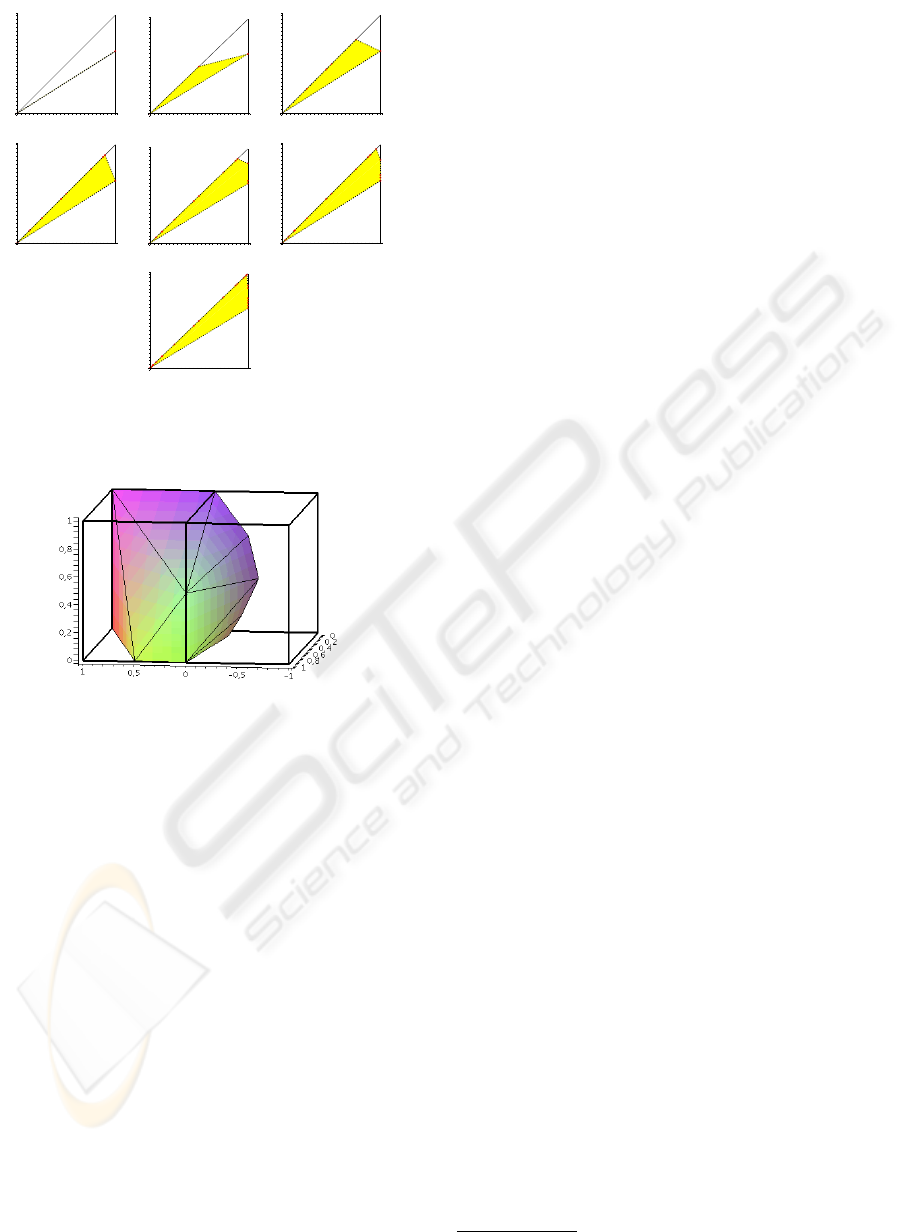
5.1 In dimension 2
We consider the linear system:
˙
X(t) =
1 1
0 1
X(t) +
−1 −2
−3 −1
u(t)
where u(t) ∈ U
2
= Conv([0, 0], [1, 0], [0, 1]). The
under-approximation algorithm is performed on the
simplex: D = Conv([0, 0], [1, 0], [0, 1]). On figure 4,
we show the successive steps to build a good under-
approximation of the controllable domain.
5.2 In dimension 3
We now consider the system for q ∈ N:
˙
X(t) =
q 0 q
0 3q 0
0 q q
X(t)+
−1 0 0
0 −2 0
0 0 −1
u(t)
with u (t) ∈ Conv([0, 0, 0], [1, 0, 0], [0, 1, 0], [0, 0, 1]).
The under-approximation is performed on two adja-
cent cubes (see figure 5) in modes (q = 0, q = 6).
6 CONCLUSION
In this paper, we addressed the optimal control prob-
lem for piecewise affine systems. We first provided a
ICINCO 2005 - SIGNAL PROCESSING, SYSTEMS MODELING AND CONTROL
298
0,20 1
1
0,8
0,8
0,6
0,4
0,6
0,2
0
0,4
0,20 1
1
0,8
0,8
0,6
0,4
0,6
0,2
0
0,4
0,20 1
1
0,8
0,8
0,6
0,4
0,6
0,2
0
0,4
0,20 1
1
0,8
0,8
0,6
0,4
0,6
0,2
0
0,4
0,20 0,60,4 1
1
0,8
0,6
0,8
0,4
0,2
0
0,20 0,6
0,2
0,4
0
1
0,8
0,6
0,8 1
0,4
0,20
1
0,8
0,8
0,6
0,60,4
0,2
0
1
0,4
Figure 4: Different steps in the under-approximation for re-
spectively h = 2, 1, 0.5, 0.25, 0.1, 0.05, 0.01
Figure 5: Under-Approximation in 3d
full algorithm to compute an under-approximation of
the controllable domain. Then the resolution of the
hybrid problem is reduced to several explicit resolu-
tions of state constraints affine optimal control prob-
lems.
This algorithm however guarantees only a local op-
timization. Next step will be to give a way to find
an optimal sequence of cells containing an optimal
trajectory. Several directions to solve this problem
include: exploration of different sequences of states,
partial numerical simulations to obtain some informa-
tions on the localization of optimal trajectories and
thus reduce the exploration. Another way could be to
replace l(X(t), u), the cost function with an admissi-
ble variable change ds = l, so that the problem comes
down to a time optimal control problem. Finding the
optimal sequence would then be to minimize the time
to reach the target.
Further developments are also a study of the approxi-
mation error and a rigorous proof of the convergence
of our under-approximation towards the real control-
lable set. Future works will include the analysis of
nonlinear dynamics:
˙
X(t) = f(X(t), u(t)) by piece-
wise affine models. The hybrid approximant is build
by linear interpolation of f at the vertices of a mesh of
R
n
× U
m
. In consequence, in each cell of the result-
ing automaton, the system is subject to mixed affine
inequalities constraints in both state and control
2
.
REFERENCES
Bardi, M. and Capuzzo-Dolcetta, I. (1997). Optimal
Control and Viscosity Solutions of Hamilton-Jacobi-
Bellman Equations. Birkauser.
Bellman, R. (1957). Dynamic Programming. Princeton
University Press.
Bertsekas, R. (1984). Dynamic Programming and Optimal
Control. Athena Scientific.
Bonnans, J. and Maurin, S. (2000). An implementation
of the shooting algorithm for solving optimal control
problems. Technical Report RT-0240, INRIA.
Bryson, A. and Ho, Y. (1975). Applied Optimal Control.
Hemisphere.
Clarke, F. H. (1990). Optimization and Nonsmooth Analy-
sis. SIAM Classics in Applied Mathematics.
Dumas, J.-G. and Rondepierre, A. (2003). Modeling the
electrical activity of a neuron by a continuous and
piecewise affine hybrid system. In Proceedings of the
2003 Hybrid Systems: Computation and Control.
Dumas, J.-G. and Rondepierre, A. (2005). Algorithms
for symbolic/numeric control of affine dynamical sys-
tems. In Proceedings of the 2005 International Sym-
posium on Symbolic and Algebraic Computation.
Fierro, R., Das, A. K., V.Kumar, and Ostrowski, J. P. (2001).
Hybrid control of formations of robots.
Girard, A. (2004). Analyse Algorithmique des Syst
`
emes hy-
brides. PhD thesis, Institut National Polytechnique,
Grenoble.
Johansson, M. (1999). Piecewise Linear Control Systems.
PhD thesis, Lund Institute of Technology.
Pesch, H. (1994). A practical guide to the solutions of real-
life optimal control problems. Parametric Optimiza-
tion. Control Cybernet.
Pinch, E. (1993). Optimal Control and the Calculus of Vari-
ations. Oxford University Press.
Pontryagin, L., Boltiansky, V., Gamkrelidze, R., and
Michtchenko, E. (1974). Th
´
eorie math
´
ematique des
processus optimaux. Editions de Moscou.
Rondepierre, A. and Dumas, J.-G. (2005). Algorithms for
hybrid optimal control. Technical report, IMAG-ccsd-
00004191, arXiv math.OC/0502172.
Zhang, J., Johansson, K., Lygeros, J., and Sastry, S. (2001).
Zeno hybrid systems. International Journal of Robust
and Nonlinear Control.
2
Work in progress, see (Rondepierre and Dumas, 2005)
PIECEWISE AFFINE SYSTEMS CONTROLLABILITY AND HYBRID OPTIMAL CONTROL
299
