A NEW HIERARCHICAL CONTROL SCHEME FOR A CLASS OF
CYCLICALLY REPEATED DISCRETE-EVENT SYSTEMS
Danjing Li §, Eckart Mayer §, J
¨
org Raisch §, ‡
§Systems and Control Theory Group, Max-Planck Institute, Dynamics of Complex Technical Systems
Sandtorstrasse 1, D-39106 Magdeburg, Germany
‡Lehrstuhl f
¨
ur Systemtheorie technischer Prozesse, Otto-von-Guericke Universit
¨
at Magdeburg
Postfach 4120, D-39016 Magdeburg, Germany
Keywords:
Cyclic systems, discrete-event systems, max-plus algebra, min-plus algebra, rail traffic.
Abstract:
We extend the hierarchical control method in (Li et al., 2004) to a more generic setting which involves cycli-
cally repeated processes. A hierarchical architecture is presented to facilitate control synthesis. Specifically, a
conservative max-plus model for cyclically repeated processes is introduced on the upper level which provides
an optimal online plan list. An enhanced min-plus algebra based scheme on the lower level not only handles
unexpected events but, more importantly, addresses cooperation issues between sub-plants and different cy-
cles. A rail traffic example is given to demonstrate the effectiveness of the proposed approach.
1 INTRODUCTION
In (Li et al., 2004), a hierarchical two-level control ar-
chitecture has been introduced for a class of discrete-
event systems (DES) without cyclically repeated fea-
tures (i.e. for systems “running only one cycle”). The
upper level of this architecture produces the time opti-
mal plan based on the event time relation represented
by a max-plus algebra model. The plan describes the
time optimal sequence of events. If an unexpected
event happens at any given time, max-plus algebra
models are simulated online on the upper level to up-
date the optimal plan and the detailed time specifica-
tion for every event. Using this information, the lower
control level acts as an implementation block.
In practice, many DES applications exhibit cycli-
cally repeated features. In this case, cooperation (and
competition) issues between different cycles have to
be addressed, which is beyond the scope of the algo-
rithm in (Li et al., 2004). To cope with this situation,
the control strategy in (Li et al., 2004) is extended.
The resulting hierarchical control scheme is depicted
in Fig.1. It is composed of a two-level structure with
an independent C/D (continuous/discrete) module. In
general, the supervisory block on the upper level will
have the goal of determining the sequence of events
which optimises the given objective function in the
cyclically repeated case. This sequence of events is
referred to as the optimal plan. The C/D module is
an interface block which transforms information from
the (continuous) plant to the timed DES framework
employed on the upper level of the proposed control
architecture.
A case study representing a simple rail traffic sys-
tem is used to demonstrate how control is realised in
the proposed framework. For this example, events
correspond to specific trains crossing specific loca-
tions within the track system. A plan specifies a se-
quence of trains and track segments where trains pass
each other. The lower control level generates veloc-
ity reference signals for the trains to implement the
plan determined by the supervisory block. The C/D
block transforms position information into event time
information. For other applications, the terms “train”
and “track (segment)” have of course to be replaced
by different ones. For example, in flexible manufac-
turing systems, “product” and “machine” can be used
instead. In a general context, “train” stands for “user”,
“track (segment)” for “resource”.
This contribution is organised as follows. Section 2
summarises how to generate the set of feasible plans
for a DES without cyclically repeated processes and
extends this method to the more general setting with
cyclically repeated features. This section also ex-
plains how the optimal plan is then chosen in an on-
line procedure. The C/D block is described in Sec-
tion 3. Section 4 explains how the plan generated
at the upper level can be implemented on the lower
level with the help of min-plus algebra. A simple case
study is given in Section 5 to illustrate the effective-
ness of the proposed approach.
30
Li D., Mayer E. and Raisch J. (2005).
A NEW HIERARCHICAL CONTROL SCHEME FOR A CLASS OF CYCLICALLY REPEATED DISCRETE-EVENT SYSTEMS.
In Proceedings of the Second International Conference on Informatics in Control, Automation and Robotics - Signal Processing, Systems Modeling and
Control, pages 30-36
DOI: 10.5220/0001182800300036
Copyright
c
 SciTePress

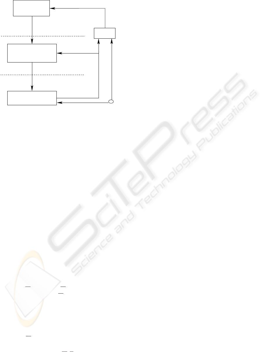
Plant
Implementation Block
(Min−plus)
lower level
plan list &
current cycles
specification for
C / D
(Max−plus model)
Supervisory Block
unexpected event
upper level
controlled variable
Figure 1: Control structure
2 SUPERVISORY LEVEL
Max-plus algebra e.g. (Baccelli et al., 1992) is a struc-
ture defined on the set IR
∗
= IR ∪ {−∞}, with max
and + as the two binary operations ⊕ and ⊗, respec-
tively. ǫ := −∞ is the additive identity in the max-
plus algebra. e := 0 is the multiplicative identity.
Based on the max-plus algebra model of the sys-
tem, the supervisory level generates the set of all fea-
sible plans (i.e. all feasible sequences of events) as
an offline task. During runtime, the supervisory level
determines the time optimal plan based on real time
information provided by the C/D module. The differ-
ence between systems with and without cyclicly re-
peated features lies in their different max-plus mod-
els. We first summarise the simpler case.
2.1 Max-plus Model for non-cyclic
Systems
Non-cyclic systems can be represented by the implicit
max-plus algebra model (Baccelli et al., 1992):
X
= A
0
⊗ X ⊕ B ⊗ u, (1)
Y = C ⊗ X
. (2)
with
A
∗
0
= I ⊗ A
0
⊗ A
2
0
⊗ · · · ⊗ A
n
0
⊗ A
n+1
0
⊗ · · · , (3)
(1), (2) can be converted to an explicit max-plus
model
X
= A
∗
0
⊗ B ⊗ u, (4)
Y = C ⊗ A
∗
0
⊗ B ⊗ u, (5)
Here, the i-th component of X
, x
i
, represents the ear-
liest possible time for event i to occur. u and Y con-
tain time information of “start” and “finish” events,
and can be interpreted as system input and output, re-
spectively.
The elements of matrix A
0
represent the minimum
time distances that have to pass between events, e.g.
(A
0
)
21
implies that event 2 may not happen earlier
than (A
0
)
21
time units after event 1 happened. In this
contribution, (A
0
)
ij
∈ IR
+
∪ {−∞, 0}. Matrix A
0
is
the max-plus sum of A
01
and A
02
, i.e.
A
0
= A
01
⊕ A
02
, (6)
where the former represents a property of the system
and is a fixed matrix, while the latter is related to the
shared resources and differs for different plans. More
specifically, the elements of A
01
represent the time re-
lation between events determined by physical proper-
ties of the system. For example, for rail systems, with
a maximum speed assumption in max-plus algebra,
the entries of A
0
represent the minimum time needed
by trains to pass distances in the network. Thus the
elements of A
01
correspond to lengths of tracks. On
the other hand, for any instance of time, a shared
track segment can only be occupied by one train. The
different occupation orders for trains on shared track
segments generate different plans. Different A
02
ma-
trices correspond to those different plans.
In a directed graph, we call the arcs corresponding
to A
01
elements “travelling arcs” while the arcs cor-
responding to A
02
elements are called “control arcs”.
For a given train track network, the travelling arcs and
therefore the entries of matrix A
01
are fixed. Fig. 2
shows the directed graph (including all possible con-
trol arcs) of a simple network with two single-line
track segments and two trains, where train 1 moves
from right to left and train 2 moves in opposite di-
rection. For single-line segment I, the control arc la-
belled a
1
, with a
1
≥ 0, represents the fact that the
earliest time instant at which train 2 may occupy this
segment is a
1
time units after train 1 has emptied
it. The control arc labelled b
1
states the reverse se-
quence. Accordingly, only one of those two arcs can
exist in any one plan. Instead of erasing a non-existent
arc from a graph, we can also label it with ǫ = −∞.
Hence, by definition, non-existing arcs have weight
ǫ. Similarly, in segment II, the arcs labelled a
2
and
b
2
represent two possibilities. Detailed information
about how to find all feasible A
02
(i.e. all feasible
plans) can be found in (Li et al., 2004). In particu-
lar, it was shown there that
∃k ≤ n, A
k
0
(i, i) > ǫ ⇔ A
02
is infeasible. (7)
2.2 Max-plus Model for Cyclicly
Repeated Systems
For system with cyclicly repeated behaviour, several
cycles may exist concurrently. Therefore, control
A NEW HIERARCHICAL CONTROL SCHEME FOR A CLASS OF CYCLICALLY REPEATED DISCRETE-EVENT
SYSTEMS
31

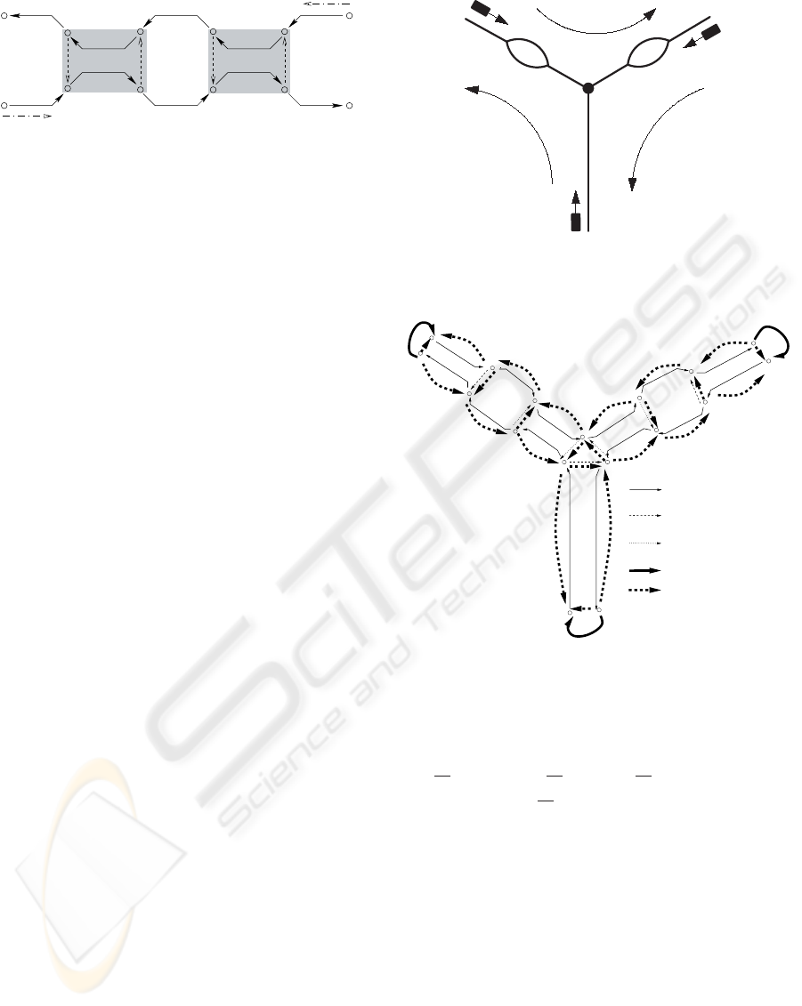
train 2
train 1
a
2
a
1
b
1
b
2
I
II
Figure 2: A network with all possible control arcs
conditions have to be extended such that trains from
different cycles will not occupy the same track seg-
ment simultaneously. Hence, additional control arcs
have to be introduced. Also, additional travelling arcs
are needed to represent the passage of trains into sub-
sequent cycles. An arc that connects events related
to the same cycle is a “zero order arc”, an arc that
connects events related to two sequential cycles is a
“first order arc”. In general, there can also be “second
order arcs” and so on. To keep our example reason-
ably simple, we introduce the following conservative
condition:
For each track segment shared by several cycles,
trains in a latter cycle may not occupy it unless all
trains in the previous cycle have left it.
With the above assumption, there is no need to in-
troduce arcs of higher order than 1. For the simple
rail traffic network in Fig. 3, which was shown in (Li
et al., 2004), “first order control arcs” ensure the safe
resource sharing between cycles and “first order trav-
elling arcs” ensure that each train starts its new jour-
ney (cycle k + 1, k ≥ 1) a specified number of time
units after its arrival at its destination in cycle k. As a
review of the example, the network involves 3 trains
and 3 tracks. Initially, train 1, 2 and 3 are located at
the end points of the 3 tracks, i.e. A, B and C, respec-
tively. The trains move along the tracks in the direc-
tions shown in Fig. 3. In the middle of both track AO
and track CO, double-line track segments are avail-
able, which make it possible that two trains pass each
other between points N
1
and M
1
or N
2
and M
2
, re-
spectively. In (Li et al., 2004), all trains stopped after
they arrived at their destinations (i.e. after one cycle).
In this contribution, each train will start a new cycle,
e.g. a given number of time units after train 1 arrived
at C, it will start the next route to go to B, which rep-
resents a new cycle. Fig. 4 shows the different kinds
of control and travelling arcs for this network. Note
that although there are optional control arcs of zero
order, all first order control arcs are fixed according to
the assumption.
Thus, for systems with cyclicly repeated behaviour,
in addition to the zero order matrix A
0
, we now have
a first order matrix A
1
. For cycle k, the implicit max-
M
1
M
2
O
A
B
C
train 1
train 2
train 3
N
1
N
2
Figure 3: A simple rail traffic network
Travelling arc for kth cycle:
zero order
Travelling arc from kth cycle
to (k+1)th cycle: first order
Control arc: first order
Fixed control arc for
kth cycle: zero order
Optional control arc for
kth cycle: zero order
Figure 4: Control arcs and travelling arcs.
plus algebra model is:
X
(k) = A
0
(k)X(k) ⊕ A
1
X(k − 1) ⊕ Bu (8)
Y (k) = C ⊗ X
(k) (9)
As for A
0
, the matrix A
1
is the max-plus sum of
two matrices A
11
and A
12
, i.e.
A
1
= A
11
⊕ A
12
, (10)
where the elements of A
11
correspond to “first or-
der travelling arcs” representing the time needed for
a train to start a new cycle after finishing the previous
cycle. The elements of A
12
correspond to the con-
trol arcs for trains belonging to two sequential cycles
respectively. Unlike A
02
, A
12
cannot represent differ-
ent choices; therefore, A
1
is a constant matrix while
A
0
will depend on the specific plan to be implemented
in the k-th cycle and is therefore varying with k.
ICINCO 2005 - SIGNAL PROCESSING, SYSTEMS MODELING AND CONTROL
32

Repeated insertion of (8) into itself provides:
X
(k) = A
0
(k) ⊗ X(k) ⊕ A
1
⊗ X(k − 1) ⊕ B ⊗ u
= A
0
(k) ⊗ [A
0
(k) ⊗ X
(k) ⊕ A
1
⊗ X(k − 1)
⊕ B ⊗ u] ⊕ A
1
⊗ X
(k − 1) ⊕ B ⊗ u
= A
2
0
(k) ⊗ X
(k) ⊕ [A
0
(k) ⊕ I] ⊗ A
1
⊗X
(k − 1) ⊕ [A
0
(k) ⊕ I] ⊗ B ⊗ u
= A
2
0
(k)X
(k) ⊕ [A
0
(k) ⊕ I]A
1
X(k − 1)
⊕ [A
0
(k) ⊕ I]Bu
.
.
.
= A
n
0
(k)X
(k) ⊕ [A
n−1
0
(k) ⊕ · · · ⊕ A
0
(k)
⊕I]A
1
X
(k − 1) ⊕ [A
n−1
0
(k) ⊕ · · ·
⊕ A
0
(k) ⊕ I]Bu (11)
As for physically meaningful systems, A
n
0
(k) will
only contain ǫ elements, the last identity represents
an explicit max-plus algebra model:
X
(k) = A
∗
0
(k) ⊗ A
1
⊗ X(k − 1) ⊕
A
∗
0
(k) ⊗ B ⊗ u (12)
Y (k) = C ⊗ X
(k), (13)
where
A
∗
0
(k) = [A
n−1
0
(k) ⊕ · · · ⊕ A
0
(k) ⊕ I]. (14)
Assume that the system input u contains initial values
of lower bounds for the state vector X(k), i.e. B = I
(B
ii
= e, B
ij
= ǫ for i 6= j), u = X in(k) (see Sec-
tion 3 for further information), (12) and (13) become
X(k) = A(k) ⊗ X(k − 1) ⊕
A
∗
0
(k) ⊗ X
in(k) (15)
Y (k) = C ⊗ X
(k) (16)
where A(k) depends on A
0
(k):
A(k) = A
∗
0
(k)A
1
. (17)
For a given system with cyclicly repeated behav-
iour, (7) can be applied to eliminate infeasible plans
and corresponding max-plus models.
2.3 Optimal Plan List
After all feasible plans have been generated, the
supervisory level may simulate feasible max-plus-
models (15), (16) over the required total number of
cycles to determine the optimal sequence of A(k),
i.e. the optimal plan list. This is initially done in an
offline fashion, i.e. before the system is started. The
objective function is typically evaluated from the out-
put vector. For example, for rail track systems, the
(offline) objective function could be
J
offline
=
min
all feasible
plan lists

L
i
Y
i
(N)

(18)
where N is the required total number of cycles and
Y
i
(N) is the arrival time of train i in the N-th cy-
cle. As ⊕ represents max, the physical meaning is
to choose the plan list giving the minimum final ar-
rival time, i.e. the minimal arrival time of the last
train in the last cycle. Since it is offline simulation,
X
in(1) only carries the starting event time. Further-
more, (X
)
i
(0) is set to ǫ = −∞. The resulting opti-
mal plan list is then implemented via the lower control
level.
Max-plus simulation in this step is obviously based
on the assumption that there is no unexpected event
and that each train either waits for a synchronisation
condition to be met or otherwise moves at its maxi-
mum velocity. Thus if any unexpected incident hap-
pens, it may affect the travelling time of trains either
directly by blocking them or indirectly via synchroni-
sation with other trains. If this happens, the runtime
event time will not match the event time calculated
by a-priori model simulation any more. To address
such difficulties, an online simulation is integrated to
update the aforementioned optimal plan list.
At time t
k
, for each of the concurrently existing
cycles l (e.g. l = k, k + 1), [X
(l)](t
k
), [Y (l)](t
k
)
will be updated by using (15), (16) with [X
in(l)](t
k
)
provided by the C/D block.
The online objective may be the same as the offline
objective (18), i.e.
J
online1
= J
offline
. (19)
It may also be different from the offline objective, for
example, it may state that after unexpected delays, all
trains have to catch up with the timetable correspond-
ing to the original offline plan list as fast as possible.
In this case,
J
online2
=
min
all feasible
plan lists
K
△
(20)
where K
△
is the index of the earliest cycle in which
all delayed trains can start (or end) their cycle trips
according to the timetable, i.e.

∀i, △
i
(l) = 0. l ≥ K
△
∃i, △
i
(l) > 0. l < K
△
(21)
△
i
(l) = t
start
i
(l) − timetable
i
(l) (22)
where t
start
i
(l) is the actual cycle starting time of
train i in cycle l, timetable
i
(l) is the cycle starting
time (according to the timetable) of train i in cycle l.
In brief, the supervisory level involves both offline
and online parts. The offline process is used to find
all feasible plans based on the system topology and
an offline optimal plan list, which can be interpreted
as a timetable. The online part updates the feasible
plan set (see (Li et al., 2004)), the optimal plan list
and provides the time specification X
(k) to the lower
level.
A NEW HIERARCHICAL CONTROL SCHEME FOR A CLASS OF CYCLICALLY REPEATED DISCRETE-EVENT
SYSTEMS
33

3 C/D BLOCK
In order to reschedule the plan (using (15)-(16)) in a
real time fashion, the state vector needs to be reini-
tialised according to the current status (at time t
k
) of
the trains for online model simulation. In other words,
the continuous variables will be transformed into a
reinitialised state vector. The reinitialised state vec-
tor X
in(t
k
) for the current cycle is:
x
in
j
(t
k
) =













x
j
if j is a past event
t
k
+ t
rest
if j is a next event,
for unblocked trains
t
rel
+ t
rest
if j is a next event,
for blocked trains
ǫ otherwise
(23)
where x
j
is the actual time at which event j happened.
t
rest
is the minimum time still needed before the next
event j may happen. It introduces continuous variable
information. For a rail track system, if a train has to
go the distance d
j
(t
k
) before it reaches the location
associated with the next event j and if the maximum
train velocity is v
max
,
t
rest
=
d
j
(t
k
)
v
max
. (24)
t
rel
is the estimated release time for the train currently
blocked. If this time cannot be estimated beforehand,
plan rescheduling will be based on the assumption of
immediate release, i.e.
t
rel
= t
k
. (25)
The supervisory level together with the C/D block
serves a model predictive control purpose, and a re-
ceding horizon concept is involved. This relates our
work to (De Schutter et al., 2002; De Schutter and
van den Boom, 2001; Van den Boom and De Schutter,
2004), where model predictive control is combined
with max-plus discrete-event systems.
4 IMPLEMENTATION LEVEL
The output of the supervisory level is the time spec-
ification X
(k) for the events of the currently exist-
ing cycles ( e.g. j = k , k + 1). X
(k) provides the
earliest possible time for each event due to the max-
imum speed assumption under max-plus. Accord-
ing to EPET (Earliest Possible Event Time) specifica-
tions, trains will always move at maximum speed, or
otherwise stop to wait until the synchronisation con-
ditions are met. This is undesirable from an energy
saving point of view. An overall optimisation ap-
proach, minimising total energy consumption for all
trains, yields a large nonlinear problem, which, at the
moment, seems unrealistic to solve. Instead, a sub-
optimal approach is used here to determine a velocity
signal separately for each train. This is done as fol-
lows:
First, a Latest Necessary Event Time (LNET) for
each train is derived as an upper bound for the event
times. For systems with non-cyclicly repeated fea-
tures, this is done in such a way that the event time of
the final event for each train according to EPET will
be met, in addition, it is also ensured that LNET does
not violate the EPET schedule of the other trains. For
systems with cyclicly repeated features, LNET should
not violate the EPET schedule of the sequential cycle.
Min-plus algebra, the dual system of max-plus alge-
bra (Baccelli et al., 1992; Cuninghame-Green, 1979;
Cuninghame-Green, 1991), is adopted to produce the
exact LNET specification.
Suppose Q(j) is the event index set for all final
events of trains in cycle j and P
m
(j) is the index set
for all events related to train m in cycle j, then at time
t
k
the LNET specifications [
X
m
(j)](t
k
) for train m
in cycle j can be calculated as
[
X
m
(j)](t
k
) = (−(A
0
(j)
∗
)
T
) ⊗
′
[XR
m
(j)](t
k
)
⊕
′
(−A
T
(j + 1)) ⊗
′
X
(j + 1) (26)
where
[(XR
m
)
i
(j)](t
k
)=

[x
i
(j)](t
k
), i∈Q(j) or i6∈P
m
(j)
+∞, otherwise.
(27)
Thus, for each train m, its EPET X
(j) and LNET
X
m
(j) are generated. Within this corridor, the ve-
locity signal can be optimised locally for each train.
Under ideal conditions, an energy optimal trajectory
results from minimising
J
m
=
Z
v
2
m
dt. (28)
For the problem of driving a train from one station
to the next, an energy optimal driving style con-
sists of four parts: maximum acceleration, speedhold-
ing, coasting and maximum breaking (Franke et al.,
2002; Howlett et al., 1994, e.g.). On a long journey
the speedholding phase becomes the dominant phase.
Then, assuming the journey must be completed within
a given time, the holding speed (i.e. the energy opti-
mal velocity) is approximately the total distance di-
vided by the total time (Howlett, 2000). In the follow-
ing, we neglect acceleration and braking effects and
suppose the velocity between two sequential events
is the straight-line velocity (i.e. speedholding mode).
Then, (28) becomes:
J
m
=
n
X
i=1
(S
i
− S
i−1
)
2
(t
i
− t
i−1
)
(29)
s.t.
ICINCO 2005 - SIGNAL PROCESSING, SYSTEMS MODELING AND CONTROL
34

t
0
= 0 (30)
t
i
= t
i−1
+
S
i
− S
i−1
v
m
(31)
t
1E
≤ t
1
≤ t
1L
(32)
t
2E
≤ t
2
≤ t
2L
(33)
.
.
.
t
(n−1)E
≤ t
n−1
≤ t
(n−1)L
(34)
t
nE
= t
n
= t
nL
(35)
where S
0
= 0, S
i
(i = 1, 2, · · · , n) is the distance
from the current position of train m to the place where
event i happens. t
nE
and t
nL
are EPET and LNET of
event n, respectively. The numerical solution gives
the energy optimal trajectory.
5 RAIL TRAFFIC CASE STUDY
The effectiveness of the hierarchical control architec-
ture proposed in the previous sections is illustrated by
a small rail traffic example which is depicted in Fig. 3.
There are 3 feasible plans in this case study (see pre-
vious work in (Li et al., 2004)).
In a first step, a fixed optimal-time plan list is de-
rived from offline simulations. The system is ex-
pected to run based on this list. If unexpected events
happen and block some train, the supervisory level
will decide whether and how to change the plan list.
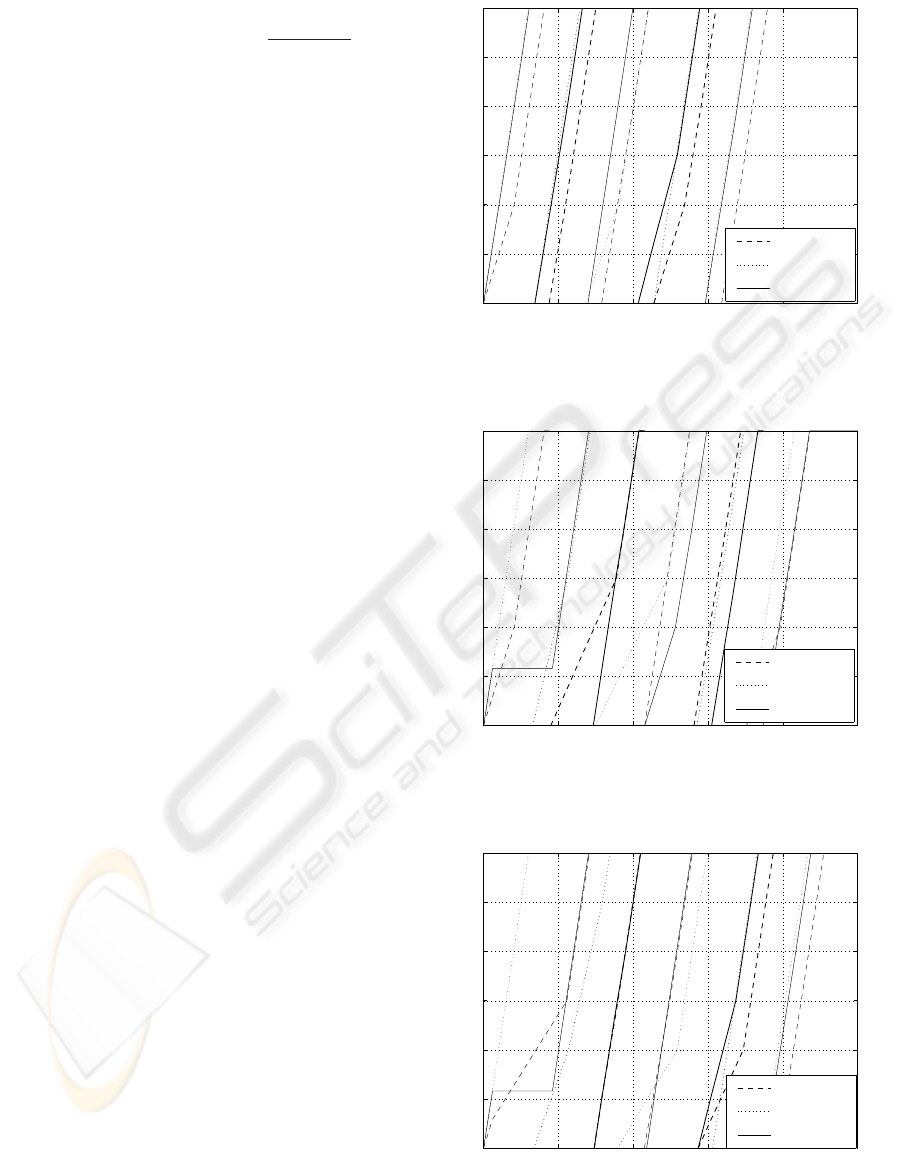
Suppose the total number of cycles is N = 5.
Fig. 5 shows the movements of the trains in a nor-
mal situation. The optimal plan list is [1 2 2 1 2].
In case of a disturbance (here train 3 is blocked on
track M
2
N
2
during the time interval [6, 46]), the su-
pervisory level checks if it is necessary to modify the
plan list using J
online1
. This scenario is presented in
Fig. 6 and Fig. 8, respectively. In Fig. 6, the blocking
time is known beforehand. With this blocking time
information, the supervisory level changes the plan
list immediately to reduce the delay time caused by
the obstacle. The required 5 cycles finish in about
219 time units. As a comparison, Fig. 7 keeps the
original plan list and the required 5 cycles finish in
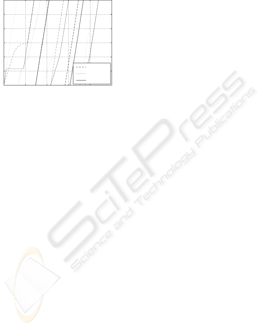
about 228 time units. If the blocking time is unknown
beforehand, the supervisory level also keeps the orig-
inal plan list until the status of the trains (include the
blocked train) evolve to such an extent that another
plan list optimises the online objective J
online1
. In
this example, as shown in Fig. 8, with the new plan
list, [1 2 1 2 2], the required 5 cycles still can finish in
219 time units.
Under the same blocking situation, with different
online objectives, the supervisory level may change
to different plan list. If, for example, the required
number of cycles is 7, and train 3 is blocked during
the time interval [6, 26], and the online cost function
0 50 100 150 200 250
0
5
10
15
20
25
30
Train 1
Train 2
Train 3
Figure 5: Simulation result under normal situation, plan list:
[1 2 2 1 2]
0 50 100 150 200 250
0
5
10
15
20
25
30
Train 1
Train 2
Train 3
Figure 6: Blocking time is known beforehand, new plan list:
[3 2 1 2 2]
0 50 100 150 200 250
0
5
10
15
20
25
30
Train 1
Train 2
Train 3
Figure 7: Blocking time is known beforehand, stick to orig-
inal plan list: [1 2 2 1 2]
A NEW HIERARCHICAL CONTROL SCHEME FOR A CLASS OF CYCLICALLY REPEATED DISCRETE-EVENT
SYSTEMS
35

0 50 100 150 200 250
0
5
10
15
20
25
30
Train 1
Train 2
Train 3
Figure 8: Blocking time is unknown beforehand, new plan
list: [1 2 1 2 2]
J
online2
is used, the supervisory level changes the
plan list from [1 2 2 1 2 2 2] to [1 2 1 2 2 2 2], and
the offline timetable is recovered after the 6th cycle.
With J
online1
, the plan list is changed to [1 2 1 2 2 1
2], which minimises the required time. However, for
this policy, the timetable is not recovered.
6 CONCLUSION
This contribution proposes a hierarchical control ar-
chitecture for a class of discrete-event systems with
cyclicly repeated features and illustrates it through a
small rail traffic example. Based on a max-plus alge-
bra model, an upper level supervisory block ensures
the optimal sequence of train movements and the op-
timal sequence of cycle plans even under disruptive
conditions. A lower level implementation block pro-
vides reference velocity signals for each train. By
exploiting the remaining degrees of freedom, it re-
duces overall energy consumption. The implementa-
tion policy is generated by use of the dual min-plus
algebra model. Simulation results for the rail traf-
fic example show the effectiveness of the approach.
We expect the method to be also useful in other DES
applications which exhibit cyclicly repeated features,
such as flexible manufacturing systems and chemical
batch processing plants.
REFERENCES
Baccelli, F., G.Cohen, G.J.Olsder, and J.P.Quadrat (1992).
Synchronization and Linearity. John Wiley and Sons,
New-York.
Cuninghame-Green, R. (1979). Minimax algebra. Springer-
Verlag, Berlin. Vol. 166 of Lecture Notes in Eco-
nomics and Mathematical Systems.
Cuninghame-Green, R. (1991). Minimax algebra and appli-
cations. Fuzzy Sets and Systems, 41:251–267.
De Schutter, B. and van den Boom, T. (2001). Model pre-
dictive control for max-min-plus-scaling systems. In
Proceedings of the 2001 American Control Confer-
ence, pages 319–324, Arlington, Virginia.
De Schutter, B., van den Boom, T., and Hegyi, A. (2002). A
model predictive control approach for recovery from
delays in railway systems. Transportation Research
Record, no.1793:15–20.
Franke, R., Meyer, M., and Terwiesch, P. (2002). Optimal
control of the driving of trains. At - Automatisierung-
stechnik, 50(12):606–613.
Howlett, P. (2000). The optimal control of a train. Annals
of Operations Research, 98:65–87.
Howlett, P., Milroy, I., and Pudney, P. (1994). Energy-
efficient train control. Control Eng. Practice,
2(2):193–200.
Li, D., Mayer, E., and Raisch, J. (2004). A novel hier-
archical control architecture for a class of discrete-
event systems. In 7
th
IFAC Workshop on DISCRETE
EVENT SYSTEMS. Reims, France, pages 415–420.
Van den Boom, T. and De Schutter, B. (2004). Modelling
and control of discrete event systems using switching
max-plus-linear systems. In 7
th
IFAC Workshop on
DISCRETE EVENT SYSTEMS. Reims, France, pages
115–120.
ICINCO 2005 - SIGNAL PROCESSING, SYSTEMS MODELING AND CONTROL
36