MULTILAYER PERCEPTRON FUNCTIONAL ADAPTIVE

CONTROL FOR TRAJECTORY TRACKING OF WHEELED

MOBILE ROBOTS

Marvin K. Bugeja† and Simon G. Fabri‡

Department of Electrical Power and Control Engineering, University of Malta

Msida MSD06, Malta

Keywords:

Wheeled mobile robots, trajectory tracking, adaptive control, neural networks, stochastic estimation.

Abstract:

Sigmoidal multilayer perceptron neural networks are proposed to effect functional adaptive control for han-

dling the trajectory tracking problem in a nonholonomic wheeled mobile robot. The scheme is developed in

discrete time and the multilayer perceptron neural networks are used for the estimation of the robot’s nonlinear

kinematic functions, which are assumed to be unknown. On-line weight tuning is achieved by employing the

extended Kalman ﬁlter algorithm based on a speciﬁcally formulated multiple-input, multiple-output, stochas-

tic model for the trajectory error dynamics of the mobile base. The estimated functions are then used on a

certainty equivalence basis in the control law proposed in (Corradini et al., 2003) for trajectory tracking. The

performance of the system is analyzed and compared by simulation.

1 INTRODUCTION

The last ﬁfteen years have witnessed extensive re-

search activity on the use of artiﬁcial neural networks

for adaptive estimation and control of nonlinear sys-

tems. Since the classical pioneering paper by Naren-

dra and Parthasarathy (Narendra and Parthasarathy,

1990), numerous neural network-based algorithms

and stability proofs have been published, covering

different types of neural networks and various system

conditions (Fabri and Kadirkamanathan, 2001; Lewis

et al., 1999; Ge et al., 1999).

Robotic systems, being inherently nonlinear and

subject to a relatively high degree of uncertainty, rep-

resent an important area where neural networks hold

much promise for effecting adaptive control. In fact,

artiﬁcial neural networks have been used extensively

for the nonlinear estimation problem in motion con-

trol of mobile robots (Fierro and Lewis, 1997; Fierro

and Lewis, 1998; Corradini et al., 2003). Mobile

robots are non-linear, multiple-input, multiple-output

(MIMO) systems. In practical environments they ex-

hibit a high degree of uncertainty in the model para-

meters and are subject to unmeasurable external dis-

turbances. These characteristics necessitate the use

of robust adaptive controllers, possibly incorporating

on-line estimation of the nonlinear functions in the

process model.

In particular, the trajectory tracking problem for

nonholonomic wheeled mobile robots has become

one of the main challenges within the automatic con-

trol research community over the last decade (Fierro

and Lewis, 1995; Fierro and Lewis, 1998; Corradini

and Orlando, 2001; Asensio and Montano, 2002; Ori-

olo et al., 2002; Corradini et al., 2003; Grech and

Fabri, 2004). This research activity is not only justi-

ﬁed by the theoretical challenges posed by this partic-

ular task, but also by a vast array of potential practical

applications in the ﬁeld of mobile robotics (Corradini

and Orlando, 2001; Ding and Cooper, 2005).

However, algorithms employing neural networks

with an on-line weight tuning facility, underpinning

the adaptation feature, are more sparse (Fierro and

Lewis, 1997; Fierro and Lewis, 1998). Moreover, the

robot models commonly encountered in related liter-

ature are considered to be deterministic and process

noise and external disturbances are often ignored.

In order to address these issues, this paper proposes

the use of on-line function estimation, taking into ac-

count process noise and external disturbances, by us-

ing a speciﬁcally formulated MIMO, stochastic model

for the trajectory error dynamics of a mobile robot. A

multilayer percpetron (MLP) neural network is used

to learn these nonlinear dynamics. The proposed sto-

chastic estimation technique used for parameter ad-

justment of the MLP network is an extension of Fabri

K. Bugeja M. and G. Fabri S. (2005).

MULTILAYER PERCEPTRON FUNCTIONAL ADAPTIVE CONTROL FOR TRAJECTORY TRACKING OF WHEELED MOBILE ROBOTS.

In Proceedings of the Second International Conference on Informatics in Control, Automation and Robotics - Robotics and Automation, pages 66-72

DOI: 10.5220/0001182200660072

 SciTePress

and Kadirkamanathan’s (Fabri and Kadirkamanathan,

1998) method for a general nonlinear class of single-

input, single-output (SISO) systems, to underactuated

MIMO robotic systems. The estimated functions are

used in the trajectory tracking control law in (Corra-

dini et al., 2003), to make the robot follow a given

reference trajectory.

The paper is organized as follows. The stochas-

tic discrete-time error dynamic model for the robot

is developed in Section 2. This is then utilized in

developing an on-line, stochastic estimator based on

MLP neural networks in Section 3. The control law in

(Corradini et al., 2003) is revisited and incorporated

with the proposed recursive weight tuning algorithm,

based on extended Kalman ﬁltering in Section 4. Sec-

tion 5 presents simulation results and is followed by a

conclusion in Section 6.

2 PROBLEM STATEMENT

This paper considers a unicycle wheeled mobile ro-

bot. The robot state is expressed as a three di-

mensional vector q, known as the pose, such that

q = [x y θ]

where (x, y) is the axle midpoint co-

ordinate and θ is the robot orientation referred to a

ﬁxed frame (Corradini et al., 2003). Similarly, a given

reference trajectory can be described by a reference

derivative vector ˙q

, composed of the reference pose

velocities ˙x

, ˙y

and

such that

˙q





˙x

˙y









cos(θ

)

sin(θ

)





, (1)

where v

and ω

are the linear and angular reference

velocities respectively. Commonly, the tracking error

vector e = [e

]

is deﬁned as

e :=





cos(θ) sin(θ) 0

− sin(θ) cos(θ) 0

0 0 1









− x

− y

− θ





. (2)

The aim is to make e converge to zero so that q con-

verges to q

. The resulting tracking error equation

modelled in continuous time is given by

˙e =





cos(e

)

sin(e

)









−1 e

0 −e

0 −1





u, (3)

where u is the velocity control input vector, given by

u = [v ω]

, where v and ω are the linear and angular

input velocities of the robot, respectively. These are

related to the velocities of the robot wheels.

Discretizing the error dynamics in (3) by using a

ﬁrst order explicit forward Euler approximation with

sampling interval T seconds and assuming that the

control input vector u remains constant over each

sampling interval, the following discrete time dy-

namic model for the trajectory error vector is ob-

tained:

= f

k−1

+ G

k−1

, (4)

where the subscript integer k denotes that the corre-

sponding variable is evaluated at time instant kT sec-

onds, and assuming that the sampling interval is cho-

sen low enough for the Euler approximation to hold.

Vector f

k−1

and matrix G

k−1

are deﬁned as:

k−1





k−1

+ T v

k−1

cos(e

k−1

)

k−1

+ T v

k−1

sin(e

k−1

)

k−1

+ T ω

k−1





(5)

k−1





−T T e

k−1

0 −T e

k−1

0 −T





. (6)

Notation-wise we will occasionally drop the time in-

dex subscript where this is obvious. Introducing a

vector of discrete random variables ε

, the error dy-

namic model in (4) is converted to the following non-

linear, stochastic, MIMO, error dynamic model:

= f

k−1

+ G

k−1

+ ε

, (7)

where ε

is assumed to be an independent, zero-

mean, white, Gaussian-distributed process, with co-

variance matrix R. This stochastic term represents

the process noise and external disturbances.

The error models in (3) and (7) are based only

on the kinematic model of the mobile base. Con-

trol schemes based on a full dynamic model would

capture better the behaviour of the robot (Fierro and

Lewis, 1997; Corradini et al., 2003) because these

take into account dynamic terms such as mass, vis-

cous damping and inertia. However, such controllers

will have more complex control laws when com-

pared with those based upon kinematic modelling

only. Moreover this complexity is increased when

considering that in practice, the values of the dy-

namic process parameters are uncertain or unknown

and may even be time varying. Such complexity

might hinder the practical implementation of these

dynamic control schemes. However, the experimental

results presented in (Corradini et al., 2003) indicate

that by combining neural networks for estimation of

uncertainty in the kinematic model and a kinematic

controller, one gets superior performance in compar-

ison to the stand-alone kinematic control case. The

estimation of uncertainty introduced in the simpler

kinematic model will compensate somewhat for the

ignored dynamic parameters, that would have other-

wise been included in a full dynamic model control

scheme with all its associated complexity.

MULTILAYER PERCEPTRON FUNCTIONAL ADAPTIVE CONTROL FOR TRAJECTORY TRACKING OF

WHEELED MOBILE ROBOTS

The work proposed in this paper supports the same

philosophy, but differs from the work presented in

(Corradini et al., 2003) in two main aspects. Primar-

ily, the estimation process developed in this paper is

on-line, enriching the controller with the adaptive fea-

ture. On-line weight tuning algorithms do not require

any preliminary off-line training (Fierro and Lewis,

1998). Consequently, on-line estimators are superior

in handling real-time applications with possible un-

foreseen variations in the process parameters; a typ-

ical scenario in mobile robotics. Secondly, we con-

sider process noise and external disturbances in our

model. These disturbances are modelled as random

processes, as shown in (7). In this manner the result-

ing control scheme is more robust in the presence of

varying process parameters, noise and external distur-

bances.

3 SIGMOIDAL MLP ESTIMATOR

Theoretically speaking, the vector of discrete func-

tions f

k−1

and the matrix of discrete functions G

k−1

composing the trajectory error model in (7) are both

known, assuming that the pose vector q is available

at each sampling interval. However, as proposed in

Section 2, neural networks will be employed for the

estimation of these functions recursively, as if they

were totally unknown. This approach is justiﬁed since

in a real robot these functions depend on the robot’s

unmodelled dynamics, time-varying parameters and

unmeasurable disturbances.

In this paper two sigmoidal MLP networks, de-

noted by NN

and NN

, for the estimation of

k−1

and G

k−1

respectively, are employed. Unlike

Gaussian radial basis function (RBF) neural networks

(Poggio and Girosi, 1990; Haykin, 1999), which are

also popular in the ﬁeld of neuro-adaptive control,

MLPs do not posses the possible advantage of linear-

ity in the parameters being estimated. For this rea-

son tuning algorithms for MLPs tend to be more com-

plex and usually result in sub-optimal estimation. On

the other hand, unlike the Gaussian basis functions

in RBFs, the sigmoidal activation functions used in

MLPs are not localized, implying that typically MLP

networks require less neurons than RBF networks for

the same degree of accuracy. This in turn means that

MLP weight tuning algorithms need to handle rela-

tively less parameters, reducing computational inten-

sity, which ultimately speeds up the overall control

loop. Naturally this is imperative in real time digi-

tal control systems. These details become more pro-

nounced when dealing with high dimensional order

systems, as in the case of WMRs, where the number

of neurons increases exponentially with the number of

systems states. This is often referred to as the curse

of dimensionality (Bellman, 1961).

Since the MLP parameters do not appear linearly

in the output equation, as will become clearer

later in the section, nonlinear stochastic estimation

techniques have to be employed. In this paper the

extended Kalman ﬁlter (EKF) (Maybeck, 1979),

is used for the recursive estimation of the MLP

networks parameters. This, along with a set of

mathematical operations, is the heart of the stochastic

online weight tuning algorithm proposed next in the

following paragraphs.

Consider the following:

• x

k−1

and x

k−1

denote the two neural network in-

put vectors of NN

and NN

respectively. A con-

stant, serving as a neuron bias input, is included in

each of these two input vectors complete deﬁned as

k−1



k−1



(8)

k−1



k−1



. (9)

• φ

and φ

are the sigmoidal activation function

vectors, representing the outputs of the correspond-

ing hidden layer, whose ith element is given by

= 1/



1 + exp(−s

)



(10)

= 1/



1 + exp(−s

)



, (11)

where s

and s

are the parameter vectors of the

ith neuron in the hidden layer, characterizing the

shape of that particular sigmoidal activation func-

tion. These sigmoidal parameter vectors form part

of the overall weight vector to be estimated, mean-

ing that each activation function is shaped recur-

sively as part of the tuning process. This detail is

responsible for the undesired nonlinear appearance

of the ﬁnal weight vector in the output equation.

• L

and L

denote the number of sigmoidal activa-

tion functions in NN

and NN

respectively.

• Let the activation function parameter vectors for

and NN

be grouped in two individual vec-

tors ˆa

and ˆa

respectively, such that

ˆa

ˆs

· · · ˆs

(12)

ˆa

ˆs

· · · ˆs

, (13)

where the symbolˆindicates that the particular pa-

rameter vector is undergoing estimation.

• The employed multilayer feedforward neural net-

work structure yields the following input-output re-

lations for the two neural networks:

k−1







ˆw

k−1

ˆw

k−1

ˆw

k−1







, (14)

ICINCO 2005 - ROBOTICS AND AUTOMATION

k−1







ˆw

k−1

ˆw

k−1

ˆw

k−1

ˆw

k−1

ˆw

k−1

ˆw

k−1







, (15)

where

k−1

and

k−1

denote the output approxi-

mates of NN

and NN

respectively. Moreover,

ˆw

represents the weight vector of the connection

between the sigmoidal activation functions and the

ith output element of NN

and similarly ˆw

rep-

resents the weight vector of the connection between

the sigmoidal activation functions and the output

element of NN

that corresponds to the (ij)th

term of

k−1

. Notation-wise φ

k−1

implies that

the activation function is evaluated for x

k−1

and

ˆa

. The same notation applies for φ

k−1

• Let us group all the parameters requiring estimation

in two vectors ˆv

and ˆv

, corresponding to NN

and NN

respectively, such that

ˆv



ˆw

ˆa



(16)

ˆv



ˆw

· · · ˆw

ˆw

ˆa



. (17)

• Let z

be the complete overall weight vector de-

ﬁned as

ˆz



ˆv

. ˆv



. (18)

• Differentiating

k−1

and

k−1

with respect to

ˆz

, yields the following closed form expressions:

∇

∂(

k−1

)

∂(ˆz

)



∇

f 1

. ∇

f 2



(19)

∇

∂(

k−1

)

∂(ˆz

)



∇

Γ1

. ∇

Γ2



(20)

where ∇

f 1

,∇

f 2

,∇

Γ1

and ∇

Γ2

are deﬁned as

follows:

∇

f 1







k−1







, (21)

where 0

denotes a zero vector having the same

length as φ

k−1

∇

f 2







· · · ˆw

1,i

(φ

− φ

· · ·

· · · ˆw

2,i

(φ

− φ

· · ·

· · · ˆw

3,i

(φ

− φ

· · ·







, (22)

where i = 1, . . . , L

and ˆw

j,i

denotes the ith el-

ement of the jth output weight vector, ˆw

. Note

also that in this equation, both φ

and x

corre-

spond to time instant (k − 1).

∇

Γ1













, (23)

where γ

and γ

are deﬁned as φ

k−1

and

k−1

respectively and 0

denotes a zero

vector having the same length as φ

k−1

∇

Γ2







· · · σ

1,i

(φ

−φ

· · ·

· · · σ

2,i

(φ

−φ

· · ·

· · · σ

3,i

(φ

−φ

· · ·







(24)

where i = 1, . . . , L

and σ

j,i

is deﬁned as

ˆw

j1,i

k−1

+ ˆw

j2,i

k−1

where ˆw

jn,i

denotes the

ith element of the (jn)th output weight vector,

ˆw

. Note also that in this equation, both φ

and

correspond to time instant (k − 1).

Assuming that, within the space of interest, the neural

network approximation errors are negligibly small

when the complete weight vector ˆz

is equal to some

unknown optimal weight vector z

∗

. This is justiﬁed

in the light of the Universal Approximation Theorem

of neural networks (Haykin, 1999). It follows that the

trajectory error model in (7) can be rewritten, using

the formulated neural networks as approximations for

k−1

and G

k−1

. The resulting model is given by

= h



k−1

, x

k−1

, u

k−1

, z

∗



+ ε

, (25)

where



k−1

, x

k−1

, u

k−1

, z

∗



k−1



k−1

, v

∗



k−1



k−1

, v

∗



k−1

, (26)

with v

∗

and v

∗

representing the optimal versions of

ˆv

and ˆv

respectively. Finally, let ∇

denote the

Jacobian matrix of h



k−1

, x

k−1

, u

k−1

, z

∗



with

respect to the weight vector z

∗

evaluated at z

∗

= ˆz

then it is clear that

∇

∂



k−1

, x

k−1

, u

k−1

, z

∗



∂(z

∗

)



∗

= ˆz



∇

. ∇



, (27)

where ∇

and ∇

are deﬁned in (19) and (20) re-

spectively. Equation (26) indicates that the unknown

weight vector z

∗

, does not appear linearly in the out-

put equation in (25). For this reason a nonlinear sto-

chastic estimator is employed in the recursive weight

tuning process detailed in the next section.

4 ADAPTIVE CONTROL

SCHEME

Having derived the stochastic model (25) for the tra-

jectory error dynamics that is dependent on the MLPs

MULTILAYER PERCEPTRON FUNCTIONAL ADAPTIVE CONTROL FOR TRAJECTORY TRACKING OF

WHEELED MOBILE ROBOTS

through

k−1

and the optimal weight vec-

tor z

∗

, it is straightforward to write down the follow-

ing nonlinear state-space equations which are used

next within the EKF algorithm (predictive mode) to

enable the recursive estimation of the neural networks

weights:

∗

k+1

= z

∗

= h



k−1

, x

k−1

, u

k−1

, z

∗



+ ε

, (28)

It is assumed that:

• The initial parameter vector z

∗

has a Gaussian dis-

tribution with some mean ¯z and covariance V.

• The process noise vector ε

is Gaussian, zero-mean

and uncorrelated in time (i.e. white).

• ε

and z

∗

are independent, implying that they are

also uncorrelated.

• The conditional density of the parameter vector

∗

k+1

is approximately Gaussian. However, it

should be emphasized that the latter is only an ap-

proximation introduced by the EKF, since the non-

linearity of the stochastic model will not conserve

the Gaussian nature in z

∗

k+1

From EKF theory (Maybeck, 1979), it follows that

the following recursive weight adjustment rules can

be employed for the estimation of the weight vector:

k+1

= P

− K

∇

(29)

ˆz

k+1

= ˆz

+ K

, (30)

where K

is the Kalman gain matrix given by

= P

∇



∇

+ R



−1

(31)

and i

is the innovations vector given by

= e

− h



k−1

, x

k−1

, u

k−1

, ˆz



. (32)

k+1

denotes the prediction covariance matrix and

represents a measure of the accuracy of the estimate

ˆz

k+1

. The initial conditions for the weight vector and

the prediction covariance are set to some desired val-

ues ¯z and V respectively.

For each estimate of ˆz

, the corresponding esti-

mates

k−1

and

k−1

are computed using the formu-

lated relations given by (8) to (18). These estimates

are then used recursively in the control law adopted

from (Corradini et al., 2003), making the overall con-

trol scheme adaptive, since the process model used

for control is now being estimated in real-time and

requires no preliminary off-line training.

Note that the extra computational burden that

comes along with the EKF, in comparison to other

non-stochastic techniques such as back-propagation,

pays off in several ways. Primarily, it renders the

recursive weight tuning algorithm stochastic, since

the uncertainty in the process model is taken into ac-

count by the EKF algorithm. Secondly, the condi-

tional probability density of the error vector e

is be-

ing updated in real time. The resulting information,

most importantly the covariance matrix P

, is essen-

tial in the design of stochastic control laws (Fabri

and Kadirkamanathan, 2001), which are part of our

plan for future work. On the other hand, it is widely

known that the assumption of local linearity inher-

ent in the EKF, may lead to convergence problems

in highly nonlinear applications. For this reason fu-

ture investigation of other nonlinear estimation tech-

niques, such as the Unscented Kalman Filter (UKF)

(Julier and Uhlmann, 1997) is desirable.

The discrete error model utilized in (Corradini

et al., 2003) is effectively given by





k−1

+ h

k−1

, v

k−1

)

k−1

+ h

k−1

, v

k−1

)

k−1

+ h

(ω

k−1

)









−T h

k−1

)

0 h

k−1

)

0 −T





k−1

, (33)

where h

to h

represent nonlinear functions, appro-

priately deﬁned in (Corradini et al., 2003). Compar-

ing (33) with the stochastic model in (7) and ignoring

the stochastic term, the following relations become

evident:

k−1

) = g

k−1

, v

k−1

) = f

k−1

− e

k−1

(34)

(ω

k−1

) = f

k−1

− e

k−1

where f

and g

denote the ith and (ij)th element

in f

k−1

and G

k−1

respectively. Hence the estimates

k−1

and

k−1

provided by the neural networks, can

be used to estimate h

, h

and h

recursively accord-

ing to (34). These are then used in the control law

proposed in (Corradini et al., 2003), given by

+ h

)ω

+ h

, v

)}

(ω

) + k

+ k

}. (35)

The design parameters k

, k

and k

can be selected

according to the following set of relations:

= 1 − λ

= 2 − λ

− λ

(36)

T v

(1 − λ

− λ

+ λ

with λ

, λ

and λ

being the eigenvalues of the re-

sulting closed loop error discrete dynamics, that must

be placed inside the unity circle to guarantee local

asymptotic stability as suggested in (Corradini et al.,

2003).

ICINCO 2005 - ROBOTICS AND AUTOMATION

5 SIMULATION RESULTS

The proposed on-line adaptive control scheme was

veriﬁed and compared to the non-adaptive scheme

proposed in (Corradini et al., 2003) by simulations.

The mobile robot was simulated through a discrete-

time model whose error dynamics were given in (7).

The covariance R of the noise vector ε

was set to

1 × 10

−6

, where I

denotes an (i × i) identity ma-

trix. Neural network pre-training is not used and, to

demonstrate further the adaptive feature of the pro-

posed controller, the model used for simulations is

abruptly modiﬁed by replacing T by 1.5T in (7) in the

middle of the simulation, speciﬁcally at 12.5 seconds.

This has the effect of modifying the robot model

considerably without altering its kinematic structure.

The selected reference trajectory was generated recur-

sively (one time step ahead) using:

(t) = 2 cos(0.25t),

(t) = 2 sin(0.5t), (37)

(t) = arctan ( ˙y

/ ˙x

) ,

which deﬁne a ﬁgure-of-eight path in the x-y plane.

Neural networks NN

and NN

were structured

with 18 and 1 hidden unit neurons respectively. The

EKF initial covariance P

was set to 5I

, where α is

the total number of weights. The initial weight val-

ues were randomly generated from a normal distrib-

ution with zero mean. The controller design parame-

ters were set according to (36) with the eigenvalues

placed inside the unity circle. Several simulation tri-

als were conducted, each indicating good tracking and

repeatable performance for the proposed algorithm.

A number of results from a particular 25 second du-

ration simulation, with a time step of 10 ms, are de-

picted in Figure 1.

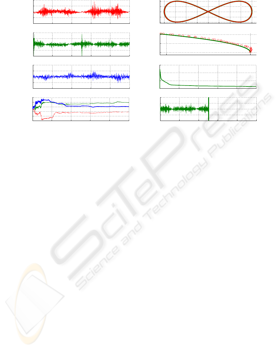
Referring to Figure 1, plots (a) to (g) were gen-

erated using the proposed adaptive controller while

plot (h) corresponds to the non-adaptive controller

proposed in (Corradini et al., 2003) under the same

speciﬁed simulation conditions and assuming that the

original robot functions are known. Primarily one

should note that the pose errors shown in plots (a),

(b) and (c) remain well bounded about zero during the

whole trajectory, indicating that the proposed scheme

has learned the nonlinear functions and yields stable

control throughout the simulation, including the pe-

riod following the previously mentioned model vari-

ation at time 12.5 seconds. This variation is over-

come with no more than a slight error transient vis-

ible in (b). This transient dies out quickly once the

controller adapts to the recently modiﬁed model. By

contrast, plot (h) reveals that the non-adaptive method

proposed in (Corradini et al., 2003) goes unstable just

after this model variation.

The complete trajectory path in the x − y plane is

superimposed on the reference trajectory in plot (e).

The two are hardly distinguishable due to the good

tracking performance obtained. The relatively high

deviation in the initial part of the trajectory, magniﬁed

in plot (f), corresponds to the learning phase of the

neural networks, which require no preliminary off-

line training.

The neural network weights remain well bounded

at reasonable values. Plot (d) depicts time plots for

three particular weights, selected arbitrarily. For these

particular simulations, the absolute maximum and

minimum weight values over the two trajectories were

8.2 and −9.4 respectively, with the majority of the

weights centred about zero. This indicates that the

proposed algorithm is also practically realizable as no

inﬁnitely high neural network weights are required.

As a result, the control velocities v and ω remained

well bounded with decent magnitudes.

Plot (g) depicts the mean of the diagonal of the co-

variance matrix P

in time. This is used to indicate

the uncertainty in the estimated weights, as generated

recursively by the EKF. As expected, the uncertainty

decreases with time, indicating that the EKF is stable

and the neural network estimations are continuously

improving. The slope of this curve is related to the

learning rate of the system.

6 CONCLUSIONS

In this paper a neural network adaptive control

scheme for the trajectory tracking problem of mo-

bile robots is proposed. The resulting algorithm re-

quires no preliminary information about the process

non-linear functions and uses MLP neural networks,

trained online in consideration of the process uncer-

tainties and external disturbances by using the EKF.

The designed scheme was tested repeatedly by simu-

lation for several noise conditions and sudden model

variations, modeling the uncertainty and time-varying

parameters encountered in practical environments. In

contrast to the non-adaptive scheme proposed in (Cor-

radini et al., 2003), the robot exhibited good tracking

performance in each case.

Future research will include the development of

stochastic non-linear control laws (Fabri and Kadirka-

manathan, 2001), which would take into account

the neural network approximation errors recursively

through the readily available covariance matrix P

Such a controller would then be amalgamated with the

estimation algorithm developed in this paper, replac-

ing the current heuristic certainty equivalence control

law. This is anticipated to give better transient perfor-

mance due to its stochastic features. Stability proofs

in the ambience of stochastic control are very rare due

to the complexity of random processes, but is still part

of our agenda for future work.

MULTILAYER PERCEPTRON FUNCTIONAL ADAPTIVE CONTROL FOR TRAJECTORY TRACKING OF

WHEELED MOBILE ROBOTS

0 5 10 15 20 25

−10

−5

(a)

− x (mm)

0 5 10 15 20 25

−20

−10

(b)

− y (mm)

0 5 10 15 20 25

−4

−2

(c)

− θ (deg)

−2 −1.5 −1 −0.5 0 0.5 1 1.5 2

−2

−1

(e)

y (m)

x (m)

1.99 2

0.2

0.4

(f)

x (m)

y (m)

0 5 10 15 20 25

(g)

Diagonal mean of P

0 5 10 15 20 25

−3

−2

−1

(d)

time (s)

Some neural network weights

0 5 10 15 20 25

−20

−10

(h)

time (s)

− y (mm)

Figure 1: Proposed algorithm: (a) error in x, (b) in y, (c) in θ, (d) some weights, (e) complete reference (—) and actual (◦)

trajectories, (f) initial phase of (e), (g) diagonal mean of P

. Non-adaptive algorithm: (h) error in y.

REFERENCES

Asensio, J. R. and Montano, L. (2002). A kinematic and dy-

namic model-based motion controller for mobile ro-

bots. In Proc. 15th IFAC World Congress on Auto-

matic Control (b’02), Barcelona, Spain.

Bellman, R. (1961). Adaptive Control Processes: A Guided

Tour. Princeton University Press, Princeton, NJ.

Corradini, M. L., Ippoliti, G., and Longhi, S. (2003). Neural

networks based control of mobile robots: Develop-

ment and experimental validation. Journal of Robotic

Systems, 20(10):587–600.

Corradini, M. L. and Orlando, G. (2001). Robust tracking

control of mobile robots in the presence of uncertain-

ties in the dynamic model. Journal of Robotic Sys-

tems, 18(6):317–323.

Ding, D. and Cooper, R. A. (2005). Electric-powered

wheelchairs. IEEE Control Systems Magazine,

25(2):22–34.

Fabri, S. G. and Kadirkamanathan, V. (1998). Dual adaptive

control of nonlinear stochastic systems using neural

networks. Automatica, 34(2):245–253.

Fabri, S. G. and Kadirkamanathan, V. (2001). Functional

Adaptive Control: An Intelligent Systems Approach.

Springer-Verlag, London, UK.

Fierro, R. and Lewis, F. L. (1995). Control of a nonholo-

nomic mobile robot: Backstepping kinematics into

dynamics. In Proc. 34th Conference on Decision and

Control (CDC’95), pages 3805–3810, New Orleans,

LA.

Fierro, R. and Lewis, F. L. (1997). Robust practical point

stabilization of a nonholonomic mobile robot using

neural networks. Journal of Intelligent and Robotic

Systems, 20:295–317.

Fierro, R. and Lewis, F. L. (1998). Control of a non-

holonomic mobile robot using neural networks. IEEE

Trans. Neural Networks, 9(4):589–600.

Ge, S. S., Lee, T. H., and Harris, C. J. (1999). Adap-

tive Neural Network Control of Robotic Manipulators,

volume 19 of World Scientiﬁc Series in Robotics and

Intelligent Systems. World Scientiﬁc Publishing Co

Pte Ltd, USA.

Grech, R. and Fabri, S. G. (2004). Trajectory tracking of a

differentially driven wheeled mobile robot in the pres-

ence of obstacles. In Proc. 12th Mediterranean Con-

ference on Control and Automation (MED’04), Izmir,

Turkey.

Haykin, S. (1999). Neural Networks: A Comprehensive

Foundation, chapter 5. Prentice Hall, London, UK.

Julier, S. J. and Uhlmann, J. K. (1997). A new ex-

tention of the Kalman ﬁlter to nonlinear systems.

In Proc. of AeroSense: The 11th Int. Symp. on

Aerospace/Defence Sensing, Simulation and Controls.

Lewis, F. L., Jagannathan, S., and Yesildirek, A. (1999).

Neural Network Control of Robot Manipulators and

Nonlinear Systems. Taylor and Francis, Padstow, UK.

Maybeck, P. S. (1979). Stochastic Models, Estimation and

Control, volume 141-1 of Mathematics in Science and

Engineering. Academic Press Inc., London, UK.

Narendra, K. S. and Parthasarathy, K. (1990). Identiﬁca-

tion and control of dynamical systems using neural

networks. IEEE Trans. Neural Networks, 1(1):4–27.

Oriolo, G., Luca, A. D., and Vendittelli, M. (2002). WMR

control via dynamic feedback linearization: Design,

implementation and experimental validation. IEEE

Trans. Contr. Syst. Technol., 10(6):835–852.

Poggio, T. and Girosi, F. (1990). Networks for approxima-

tion and learning. Proc. IEEE, 78(9):1481–1497.

ICINCO 2005 - ROBOTICS AND AUTOMATION