
A HYBRID CONTROLLER FOR A NONHOLONOMIC
CAR-LIKE ROBOT
Martin v. Mohrenschildt
McMaster University
Factulty of Engineering, Hamilton, Canada
Keywords:
Hybrid Systems, Switched Systems, Finite Horizon Control, Supervisory Control, Nonholonomic robot.
Abstract:
This paper presents the usage of hybrid systems to develop an adaptive recent horizon controller for a nonholo-
nomic car-like robot. The system is modeled by a non-deterministic hybrid system in which transitions repre-
sent the discrete control actions, mode invariants the constraints and the transition relation encodes sequencing
requirements. The control algorithm examines at runtime the possible traces into the future by determining at
which time point to switch to which mode. Based on these predictions the next control move is performed. We
demonstrate our approach by controlling a car-like robot though a maze without any pre-runtime path planing.
1 INTRODUCTION
In many applications a high level digital controller is
interacting with a set of low level controllers and actu-
ators. Often these low level controllers and actuators,
being for example PID controllers, accept only a finite
set of discrete control actions, e.g. start PID controller
i, turn left, open valve. While there is a finite num-
ber of possible control actions, the control input itself
is continuous. For a car the actions are turn steering
wheel left, turn it right or hold it at its current position,
accelerate, hold speed, de-accelerate. Clearly, there
are constraints, the steering wheel can only turned
right until it reaches its maximal right position, ac-
celeration and de-acceleration rates are finite.
Such control systems can perfectly be modeled us-
ing hybrid systems (Almeida et al., 1997; Abdelwa-
hed et al., 2002; Kowalewski et al., 2000; v. Mohren-
schildt, 2001; Abdelwahed et al., 2002; Labinaz et al.,
1997; Bemporad et al., 2000; Bemporad and Morari,
1999). A hybrid system has continuous states that
evolve according to differential equations, and a fi-
nite set of modes that evolve according to transitions.
Changing mode causes a discrete change of the dif-
ferential equations. The transitions in between modes
are be guarded by conditions on the state variables.
Further, each mode contains a mode invariant, a predi-
cate on the state variables that has to remain true while
the system is in that mode. These hybrid systems are
non-deterministic in their transitions, a transition can
occur if its guard allows it, but some transition has to
occur if the invariant in a mode becomes false. The
goal of the control algorithm is to trigger the tran-
sitions, at runtime, such that the system exhibits the
desired behavior; minimizing some cost function J.
The controller proposed in this paper is adaptive in the
sense that the control frequency, the amount of time
in between control moves, is not fixed but changes.
If becomes shorter as there are constraints and longer
otherwise. The control algorithm bases its decision
on predictions of the future behavior of the system.
As found in many systems in nature, a human driving
a car, the control algorithm sees the constraints, being
walls or bends in the road only within a finite predic-
tion horizon.
The approaches presented in (Almeida et al., 1997),
the authors develop a hybrid controller to control a
non-holonomic vehicle that inspired us to apply our
approach to motion control problems, and (Abdelwa-
hed et al., 2002; Kowalewski et al., 2000) develop-
ing a controller for a two tank system, relaying on a-
priory analysis of the control problem to develop there
hybrid systems. In contrast, the constructions of our
controller is generic, resulting in a non-deterministic
hybrid system, only the prediction horizon has to be
determined by analyzing the system to be controlled.
The transition conditions that define the control strat-
egy are determined at run time by the supervisor al-
gorithm.
Several questions arise: Can the control algorithm
282
v. Mohrenschildt M. (2005).
A HYBRID CONTROLLER FOR A NONHOLONOMIC CAR-LIKE ROBOT.
In Proceedings of the Second International Conference on Informatics in Control, Automation and Robotics - Signal Processing, Systems Modeling and
Control, pages 282-288
DOI: 10.5220/0001175802820288
Copyright
c
SciTePress

prevent the system from entering a blocking state,
does the control algorithm control the system into its
global minimum with respect to the cost function or
do we get stuck in some local minimum. We show
that under some general assumptions the proposed
control algorithm can satisfy both of these goals. The
approach taken follows the ideas presented in (Mayne
and Michalska, 1990; Primbs and Nevistic, 2000;
Almir and Bornard, 1995) by choosing a prediction
horizon such that the finite horizon controller is stabi-
lizing.
We apply the proposed approach to the problem of
controlling a non-holonomic car-like robot. The goal
of the algorithm is to control a robot though a maze.
The algorithm does not have a map of the maze, nei-
ther is there any pre-runtime motion planing. The al-
gorithm can only explore the maze within a limited
horizon of its current position. We show simulations
using a tracked vehicle, a vehicle that can turn on a
dime, and a car-like wheeled vehicle. The simula-
tions where performed using a generic implementa-
tion of the developed control algorithm in conjunction
with C-code that was automatically generated using
the computer algebra system Maple from the sym-
bolic solutions of the differential equations.
First we introduce the hybrid systems used to
model the system. Section 4 presents the control algo-
rithm and investigates stability conditions. In section
5 we then apply our control algorithm to steer a car-
like robot though a maze.
2 HYBRID SYSTEMS, EVENTS,
CONTROLLED TRACE
A vast amount of literature contains detailed dis-
cussion with different approaches to hybrid systems.
(Branicky, 1998; Gollu and Varaiya, 1989; Henzinger,
1996; Labinaz et al., 1997).
To motivate the use a non-deterministic hybrid sys-
tem as a model for control systems we give a simple
example of the movements of the steering wheel in a
car. The position of the steering wheel is given by the
angle φ, where
−π
4
≤ φ ≤
π
4
. The steering wheel
can either be turned left, turned right or held at its po-
sition. The turning rate of the steering wheel is lim-
ited:
˙
φ = −0.01,
˙
φ = 0,
˙
φ = 0.01. The hybrid sys-
tem hence has three modes: TWL,STOP,TWR, turn
wheel left, stop, turn wheel right. The turning left and
turning right modes have invariants that ensure that
the wheel is not turned to far: I(TWL) = φ ≥
−π
4
and I(TWR) = φ ≤
π
4
. In each mode φ is computed
by a differential equation: F (STOP) :=
˙
φ = 0,
F (TWL) :=
˙
φ = −0.01, F (TWR) :=
˙
φ = 0.01.
The transition guards are shown in the graphical rep-
resentation Figure 1. Note, that if the system is in the
TWL mode and φ reaches
−π
4
then the system has a
forced transition to the STOP mode. Any trace of
this hybrid system represents a “legal” motion of the
steering wheel.
Figure 1: Steering Hybrid System
Definition 2.1 (Hybrid System) A hybrid system is
a tuple
HS = (Q, X, Y, V, F, δ, I, G, A)
where:
• Q = {q
0
, q
i
, · · · , q
e
} is the set of discrete states,
called modes, of the system, X ⊆ R
n+m
is the set
of the continuous states, called states, Y ⊆ X, Y ∈
R
m
is the output space.
• V is the set of variables. We distinguish two type
of variables, state variables x
i
, 1 ≤ i ≤ n and
output variables u
i
, 1 ≤ i ≤ m, that are also state
variables.
• F : Q → (X → X) gives a set of differential
and algebraic equations that describe the continu-
ous behavior of the system for each mode.
• δ ⊆ (Q×Q) is the transition relation that describes
the discrete behavior of the system.
• I : Q → (X → bool) gives an invariant for each
mode.
• G : (Q × Q) → (X → bool) is the transition
guard function.
• A : (Q × Q) → (X → X) is the transition action.
Our systems are autonomous, transition time points
are measured relative to the start of the system, all
differential equations are autonomous. In the follow-
ing we use q
i
1
, q
i
2
, · · · to denote a sequence of modes
with indices i
1
, i
2
, · · · . An execution ǫ of the hybrid
system HS starting at some time point t
0
1
, mode q
0
and state x
0
is a sequence
ǫ = (q
0
, t
0
, Φ
0
), (q
i
1
, t
1
, Φ
1
), · · ·
such that (q
i
j
, q
i
j+1
) ∈ δ, Φ
j
(t) is the solution of the
equations F (q
i
j
) for t
j
≤ t ≤ t
j+1
, with initial con-
ditions Φ
j
(t
j
) = Φ
j−1
(t
j
), j > 0, and Φ
0
(t
0
) = x
0
.
1
This time is relative to the start of the system, the sys-
tem itself is autonomous
A HYBRID CONTROLLER FOR A NONHOLONOMIC CAR-LIKE ROBOT
283

Further it must hold that I(q
i
)(Φ
t
j
(t)) = true for
t
j
≤ t < t
i+j
, G(q
i
j
, q
i
j+1
)(Φ
j
(t
j
)) = true, and
A(q
i
j
, q
i
j+1
)(Φ
j
(t
j
))) = Φ
j+1
(t
j
).
A trace τ starting at time t
0
in mode q
0
and state
x
0
is a (finite or infinite) sequence of modes together
with the time points at which the system switched into
that mode:
τ = (q
0
, t
0
), (q
i
1
, t
1
), (q
i
2
, t
2
), · · ·
such that there is a unique execution ǫ with the same
modes and times.
As noted, the hybrid systems 2.1 are non-
deterministic. This means that the set of all traces
starting in some mode q
0
, state x
0
, and time t
0
, de-
noted with T
q
0
,x
0
,t
0
, can contain more then one ele-
ment, it is in general infinite.
There could be traces that end in a blocking state,
meaning a mode q and state x where I(q)(x) =
false and ∀˜q. (q, ˜q) ∈ δ → G(q , ˜q) = false.
Also, there could be so called zeno traces, traces
where lim
i→∞
t
i+1
− t
i
→ 0.
A transition is called a forced transitions if it hap-
pens at a time point t in some mode q and state x
where I(q)(x(t)) is false and G(q, q
′
)(x(t)) =
true.
We call a hybrid system proper if all forced tran-
sitions are unique: if the system is in the mode q,
state x at time point t and I(q)(x(t)) = false then
there exists at most one q
′
such that G(q, q
′
)(x(t)) =
true.
Definition 2.2 (Event) Given a hybrid system HS
and a set of traces T
q
0
,x
0
,t
0
. An event e
q
i
,q
j
,t
is a
mapping from the set of traces to the set of traces
that selects all the traces τ
i
∈ T
q
0
,x
0
,t
0
containing
the transition from q
i
to q
j
at time point t. the set of
all traces that change mode from q
i
to q
j
at time point
t.
Note, e
q
i
,q
j
,t
(T
q
0
,x
0
,t
0
) could be the empty set.
Finally, we can define the notion of a controlled
trace, being the set of traces in which all transitions
are either forced of are caused by an event.
Definition 2.3 (Controlled Traces) To a sequence of
events < e
q
i
j
,q
i
j+1
,t
j
>, the set of traces τ with
τ ∈ T
q
0
,x
0
,t
0
, if they exists, that contain only forced
transitions and transitions caused by the events is
called a controlled traces.
Lemma 2.4 For a proper hybrid system HS, a se-
quence of events and a set of traces the controlled
trace, if exists, is unique.
The proof consists of applying the definitions. All
forced transitions are deterministic by the properness
assumption, all other transitions in a controlled trace
correspond to events.
3 THE CONTROL PROBLEM
Equipped with hybrid systems we now model the con-
trol system by combining the model of the plant, con-
straints of physical and logical nature, and the possi-
ble control inputs, given in form of control functions,
into one hybrid system.
The system to be controlled is represented by the
system of differential equations
˙x = f(x, u)
(1)
where x ∈ R
n
, u ∈ R
m
, f : R
n
× R
m
→ R
n
models
the dynamics of the plant. We assume that the plant
is totally observable and hence, for simplicity, do not
have an explicit output function. Further the system
is assumed to be controllable and f(0, 0) = 0, and f
is Lipschitz continuous with constant L
||f(x, u) − f(˜x, u)|| ≤ L||x − ˜x||.
The control input u can not be chosen freely, but
the value of u is computed by a member of a set of
control functions cf
i
, i = 1 · · · k, cf : R
n
→ R
m
,
(Morse, 1993), the control algorithm plays the role of
a supervisor and determines the time points when to
use which controller. For one of the cf
i
it holds that
cf
i
(0) = 0. This is motivated by systems in which
digitally controlled actuators interact with the plant.
The state and the control input are constrained. The
constraints are given in form of a system of equali-
ties and inequalities. We do not restrict to linear con-
straints, since we intend to solve a non-convex prob-
lem. To model the movements of a car in a maze
we need to include the dimension of the car, collision
with walls is determined by deciding if a given set of
equalities and inequalities does not have a solution.
There could also exist logical constraints, constraints
that dictate sequencing requirements such as ˙u should
be zero before u can change from positive to negate,
e.g. the car can not reverse before it came to a com-
plete stop.
The goal of the control algorithm is to minimize the
cost function
J
t
(x, u) =
Z
t
0
g(x, u)dt
for a positive definite function g. It holds that
g(0, 0) = 0. The control algorithm is restricted in
that it does not have a global view of all constraints,
but can only see constraints that are “visible” within
a given control horizon H. This horizon can not be
chosen freely, it must by sufficiently large such that
the resulting recent horizon controller is stabilizing
(Almir and Bornard, 1995). We examine this further
in 4.1.1.
The control problem is modeled using a hybrid sys-
tem with k modes. (k is the number of control func-
tions.) In each mode the equations F (q
i
) are given
ICINCO 2005 - SIGNAL PROCESSING, SYSTEMS MODELING AND CONTROL
284

by the model equation ˙x = f (x, u) and the equa-
tion u = cf
i
(x). The mode invariants model the
constraints. The transitions encode the sequencing
requirements and the transitions are guarded by the
mode invariant they lead to. This is to ensure that
the system does not switch into a mode in which the
invariant is false. Note, for technical reasons, each
mode q
i
contains a self transition δ(q
i
, q
i
) guarded
by the invariant of the mode. To ensure that the con-
trol system remains at least a minimal amount of time
t
min
, minimal holding time, in each mode we add
the state variable, clock, with the differential equa-
tion
˙
clock = 1 to each mode, each transition guard
is augmented with clock > t
min
and t
min
is set to 0
during each transition by A. The developer has to en-
sure that the constructed hybrid system is proper by
determining which transition should be taken in case
a mode invariant becomes false and modify the tran-
sition guards accordingly.
The resulting hybrid system is called the controlled
hybrid system CHS. The control problem hence is
reduced to “switching the mode of the CHS system
at runtime”.
For convenience, for any trace τ ∈ T
q ,x,t
we write
J(τ) to denote the cost J computed over the trace τ .
The value of J(τ) can be computed over each trace
since x and u are state variables.
The control problem can not be solved in general.
We need assumptions under which an algorithm will
succeed.
Assumption 1 For x
0
and q
0
the CHS is non-
blocking, there exists an trace τ of infinite length.
For a system CHS, the set of the non blocking
traces is denoted with NBT
∞
. The infinity stands for
the fact that the set NBT
∞
could be constructed by
an infinite construction. The optimal solution of the
control problem is the trace τ ∈ NBT
∞
with minimal
J(τ) denoted as τ
∗
.
Definition 3.1 (CHS Control Problem) Given a hy-
brid system CHS, an initial state x
0
, initial mode q
0
and the cost function J, if NBT
∞
is not empty then the
sequence of events < e
q
i
j
,q
i
j+1
,t
j
> that corresponds
to τ
∗
is the optimal solution of the CHS control prob-
lem.
By construction the control hybrid system CHS re-
mains for at least t
min
time units in each mode.
4 THE CONTROL ALGORITHM
For discrete systems, recent horizon control algo-
rithms approach the problem by repeatedly solving
a finite horizon control problem, realizing the first
control move and then repeating the procedure. We
construct an equivalent process for our mixed discrete
continuous system.
As noted, the control algorithm can not explore the
entire future behavior of the system but is restricted to
the prediction horizon H.
Definition 4.1 (H-Predictive Trace) Let CHS be a
hybrid system. A H-predictive trace starting in mode
q, and state x and time point t is a trace τ =
(q, t), (q
i
1
, t
1
), · · · (q
i
n
, t
n
) of the CHS hybrid sys-
tem starting in mode q, state x and has duration H,
t
n
= t+H. The set of all these traces is denoted with
T
H
q ,x,t
.
In general the set T
H
q ,x,t
is infinite. In practice we
have to impose restrictions such that we can explore
this set. We use two constants: (1) The previously
defined t
min
, which is the minimal amount of time
the system has to remain in each of the modes in any
trace. The reason to restrict the minimal amount of
time the system has to remain in a mode to t
min
is to
gives us the time needed to run the control algorithm.
(2) t
max
, which is the maximal amount of time the
system can remain in any mode without considering
to switch mode. t
min
,t
max
gives us the time frame in
which control moves are scheduled to happen. These
restrictions now allow us to reduce the size of T
H
q ,x,t
:
Definition 4.2 (Restricted H-Predictive) A re-
stricted H-predictive trace starting in mode q and
state x is a predictive trace
τ = (q, t), (q
i
1
, t
1
), (q
i
2
, t
2
), · · · (q
i
n
, t
n
)
where t
k+1
− t
k
, the time spend in mode q
k
, is
uniquely determined as the maximal amount of time
the system can remain in mode q
i
k
while the invariant
I
q
i
k
holds and t
min
≤ t
k+1
− t
k
≤ t
max
.
By construction we have t
k+1
− t
k
≥ t
min
.
Note, the CHS hybrid system contains self transi-
tions for each mode, this means in a predictive trace
the system could remain in any mode as long as the
invariant of this mode is not violated. We use RT
H
q ,x
to denote the set of all restricted H-predictive traces
that start in mode q and state x By construction and
lemma 2.4, RT
H
q ,x
is a finite set. Transitions either cor-
respond to events or are forced. The length n of the H
predictive traces is at most xH/t
min
y and the at least
xH/t
max
y.
Now we are ready to give the control algorithm:
Definition 4.3 (Supervisor) Let t
i
be the next time
point where a control move is required, and t
run
be
a constant given at the end of this definition.
1. At time point t
i
−t
run
the supervisor reads the mode
q and state x of the system and determines all re-
stricted H-predictive traces RT
H
x,q
:
τ = (q, t
i
− t
run
), (q
i
1
, t
i
), (q
i
2
, t
2
), · · · (q
i
n
, t
n
)
A HYBRID CONTROLLER FOR A NONHOLONOMIC CAR-LIKE ROBOT
285

which are the traces that start in mode q remain for
t
run
in mode q and then switch to some new mode
q
i
1
, which could be q again.
2. If RT
H
x,q
is the empty set, meaning there is no con-
trol move that prevents the violation of the con-
straints the system has to be stopped or invoke a
user defined ad hoc procedure to relax constraints
so that the system becomes feasible again. Let
τ be the trace with minimal J(τ) of the traces
τ ∈ RT
H
x,q
.
3. At time point t
i
the supervisor causes the hybrid
system to switch to the mode q
i
1
.
4. The supervisor waits until the time point t
2
− t
run
and starts again with step 1.
t
run
is the amount of time the supervisor needs to per-
form its computation.
The algorithm should also keep track of the value of
J(τ) computed in the previous step and check that it
is larger then J(τ) computed in the current step which
allows to verify that the plant progresses towards the
minimum of J as detailed in the next section.
4.1 Stability and Complexity
There is a documented gap between the theoret-
ical stability results for recent horizon controllers
and there practical use in industrial applications
(Allg
¨
ower and Findeisen, 2002; Morari and Lee,
1999; Davrazos and Koussoulas, 2001). Stability is
assured by either introducing carefully chosen ter-
minal weights, defining a set that has to be reached
within each of the finite predictions, or by determin-
ing the prediction horizon such that repeatedly solv-
ing the finite horizon problem results in a global op-
timal solution (Mayne and Michalska, 1990; Primbs
and Nevistic, 2000; Almir and Bornard, 1995). We re-
lay on the latter approach by determining assumptions
under which the proposed algorithm is stabilizing.
4.1.1 Stability
To show stability of the proposed control algorithm
we relay on the classic Liapunov argument using the
costs J
H
(x, q) computed over the finite horizon H,
which are the predictive traces, as Liapunov function
(Mayne and Michalska, 1990; Primbs and Nevistic,
2000; Almir and Bornard, 1995). We have to de-
termine under which conditions the sequence of the
J
H
(x, q) is decreasing.
To ensure convergence we assume that the pre-
diction horizon is sufficiently large such that the se-
quence of the costs J(τ
i
) where τ
i
is the predictive
trace computed in the i-th step of the control algo-
rithm is decreasing.
Assumption 2 For all traces
τ = (q
0
, t
0
), (q
i
1
, t
1
), (q
i
2
, t
2
), · · ·
starting in state x
0
and mode q
0
, with τ ∈ NBT
∞
,
there is an H such that for all the finite traces ˜τ ∈
RT
H
q
j
i
,x
i
and
τ ∈ RT
H
q
j
i+1
,x
i+1
, ˜τ and τ being the op-
timal traces, where x
i
is the i-the state and q
j
i
the i-th
mode of τ, there is an α, 0 < α < 1 such that
αJ(˜τ) ≤ J(
τ).
Assumption 2 ensures that the finite horizon strat-
egy can succeed in solving the control problem by re-
quiring that H was choose such that for all predictive
traces τ
i
sup
J(τ
(
i + 1))
J(τ
i
)
< 1.
This represents the conditions of the stability criteria
as found in the above mentioned literature.
Let τ be the trace and ǫ be the corresponding exe-
cution. To apply the stability criteria we translate our
continuous system into a discrete sequence of states
by using the solutions Φ
i
of the execution, hence
x(n + 1) = Φ
i
(x(n), t
n+1
)
This sequence is well defined since the solution to the
initial problems as we enter mode q
i
n
is unique.
Theorem 4.4 (Stability) Under the assumptions 1,2
the control algorithm is stable.
We have to show that repeatedly computing the pre-
dictive traces, determining a sequence of events we
obtain a trace that approximates the optimal solution
τ
∗
of the control problem. Let τ
i
be the sequence of
the predictive traces choose by the control algorithm.
Let x(j) and q
i
j
be the state and mode we are in at
time point t
j
, j = 0 is the initial state. q
i
j+1
is de-
termined from the trace ˜τ ∈ RT
H
q
j
i
,x(i)
with minimal
cost. The system moves to mode q
i
j+1
at time point
t
k+1
where we are in state x(j + 1). Let
τ be the next
traces determined by the algorithm 4.3. Be assump-
tion 2 we have that either that J(τ ) < J(˜τ) since
α < 1, or they are equal in the case that we already
reached the stable point x = 0. By this the cost of the
local finite horizon predictions as computed by the al-
gorithm J(τ
i
) is decreasing and with this the system
is stable.
4.1.2 Complexity
The complexity of our approach is determined by the
size of the set RT
H
q ,x,t
which grows exponentially in
the number of mode switches of the predictive traces.
However, in practical applications the situation is not
as bad as it first seems. If there is no “constraint vis-
ible” within the prediction horizon the predictor uses
ICINCO 2005 - SIGNAL PROCESSING, SYSTEMS MODELING AND CONTROL
286
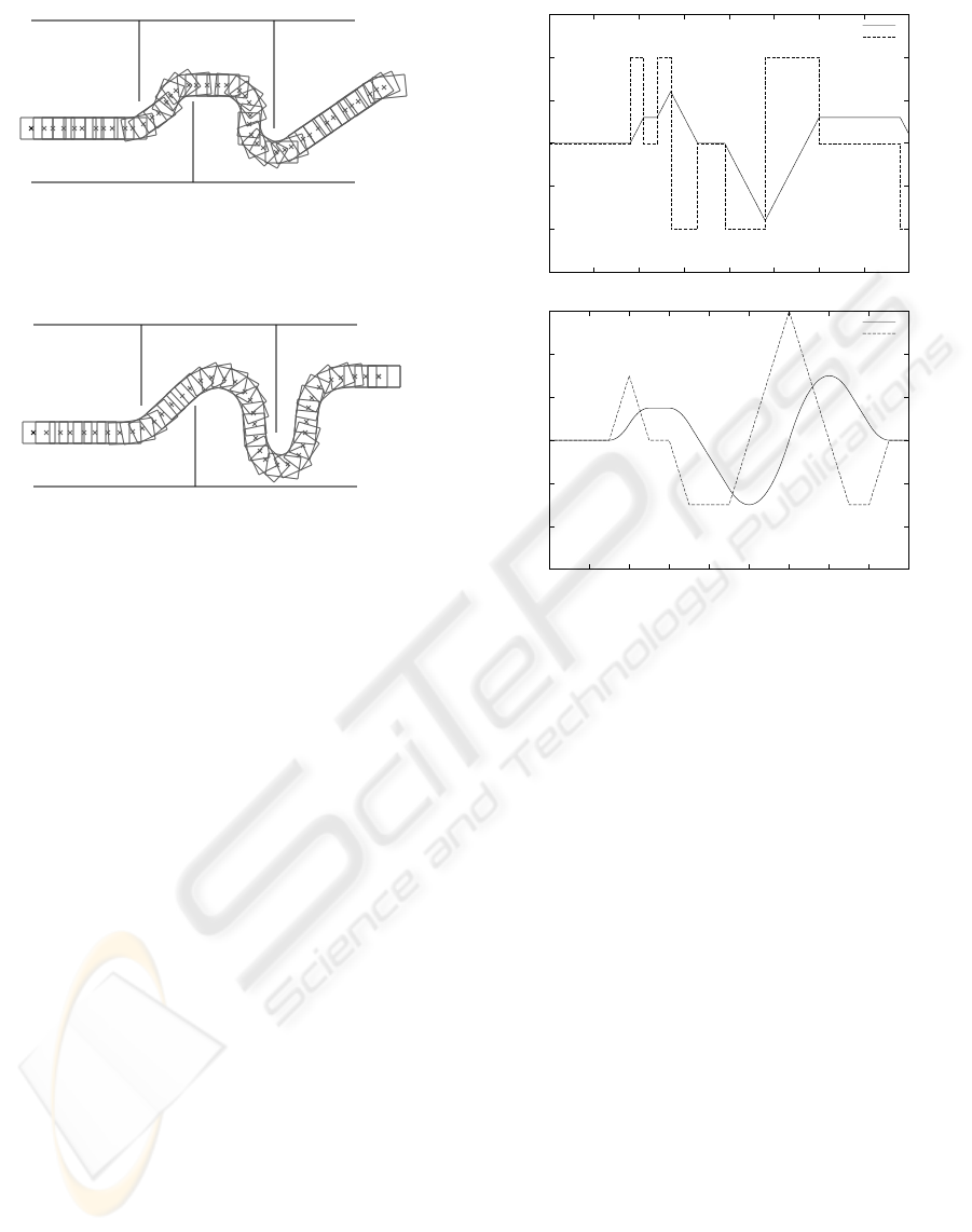
Figure 2: Track vehicle
Figure 3: Wheeled vehicle
large steps, defined by t
max
, to reach the prediction
horizon. If there are constraints then traces resulting
in a blocked state are cut reducing the search space.
The observation of the reduction in search space
caused by cutting branches of the search tree is con-
sistent with observations made by other approaches to
model predictive control (Abdelwahed et al., 2002),
(Hadj-Alouane et al., 1994). Also, our implementa-
tion uses symbolic techniques based on (v. Mohren-
schildt, 2001), which we do not detail here, that re-
duce the amount of computation needed at run-time
by symbolically pre-computing the solution of the dif-
ferential equations whenever possible. The symbolic
solutions allow us to reduce the real- time computa-
tion to evaluation of formulas. Obviously, the num-
ber of formulas is still exponential with is consistent
with the explicit MPC algorithm algorithm presented
in (Bemporad et al., 2002).
5 NONHOLONOMIC CAR-LIKE
ROBOT
We used our approach to control a nonholonomic ro-
bot moving in a maze. We present both, a car with
tracks and a car with wheels. For details about the
modeling and control of nonholonomic cars the reader
is referred to the book (Laumond, 1998). The exam-
ple presented here was inspired by (Almeida et al.,
1997).
-3
-2
-1
0
1
2
3
0 1 2 3 4 5 6 7 8
Car Angle
Turning Rate
-3
-2
-1
0
1
2
3
0 1 2 3 4 5 6 7 8 9
Car Angle
Turning Rate
Figure 4: Control input and angle for tracked and wheeled
vehicle
First we like to point out that in contrast to many
approaches to car control there is no path planing,
meaning that the car is not tracking a predefined path.
The controller can only explore the possible paths
within the prediction horizon and “sees” the walls
only as they enter into the prediction horizon. Also,
in contrast to (Almeida et al., 1997) we did not de-
velop a special controller for this problem but run the
controller as defined in this paper in its generic form.
The example demonstrates that our control algo-
rithm is able to perform point-to-point motion con-
trol without path planing. The prediction horizon H
was chosen such that the controller was able to “look
around the corner”, which means, as we move with 1
m/sec and the longest wall is 1m long we use a pre-
diction horizon of H = 1sec.
The car is modeled as follows:
˙x = v cos(θ), ˙y = v sin(θ),
˙
θ = vu
(2)
with the control variable u and v ∈ {−1, 0, 1}. x, y
is the position of the center of the rear steering axle,
θ is the rotation of the car in relation to the coordi-
nate system. The four sides of the car are computed
at runtime using x, y, θ, using the the car length .7,
width .4, and offset .2 of the rear axle.
We performed two types of simulations, u being
discrete valued, u ∈ {−2, 0, 2}, which models the
A HYBRID CONTROLLER FOR A NONHOLONOMIC CAR-LIKE ROBOT
287

movement of a track vehicle, and u being change rate
constrained, u ∈ [−3, 3], du ∈ {−5, 0, 5}, which
models a car more realistically. We extended the con-
straints for u for the wheeled car from 2 to 3 since
else the car was not able to turn sufficiently fast.
For both simulations we used a mixed numeric,
symbolic approach. To detect if the car is hitting a
wall, which means solving 4 linear systems, we gen-
erated symbolic code using the computer algebra sys-
tem Maple. We also solved the model equations sym-
bolically, but to predict the time which we can remain
in a mode, we use numeric methods. We control the
car to move to the point (7, 2), which is at the right
side middle of the maze in the figures 2.
The Figures in 2 show the movement of the car.
The first figure plots the movement of a track vehicle,
second of a car like vehicle. Figure 4 plots the con-
trol input being the change of the turning rate of the
car versus the angle of the car again for the discrete
control input and for the change rate limited control
input.
6 CONCLUSIONS
We presented an approach to model the influence of
discrete control moves using hybrid systems and pre-
sented a control algorithm. In contrast to other ap-
proaches we use a continuous model of the plant, the
continuous control input is computed my a member
of the control functions. The presented algorithm is
adaptive in the sense that the control frequency, the
frequency at which control actions occur is not fixed
but changes with the presence of constraints.
The controller was implemented for several case
studies, not limited to the here presented maze track-
ing problem, and we found that we could solve com-
plex control tasks using our generic controller.
REFERENCES
Abdelwahed, S., Karsai, G., and Biswas, G. (2002). Online
safety control of a class of hybrid systems. IEEE 2002
Conference on Decision and Control.
Allg
¨
ower, F. and Findeisen, F. (2002). An introduction to
nonlinear model predictive control. IST Technical Re-
port 2002-1.
Almeida, J. M., Pereira, F. L., and Sousa, J. B. (1997).
A hybrid system approach to feedback control of a
nonholonomic car-like vehicle. In 5th IEEE Mediter-
ranean Conference on Control and Systems, Cyprus.
Almir, M. and Bornard, G. (1995). Stability of a trun-
cated infinite constrained recending horizon scheme:
the general discrete nonlinear case. Automatica,
31(9):1353–1356.
Bemporad, A., Borrelli, F., and Morari, M. (2000). Optimal
controllers for hybrid systems: Stability and piecewise
linear explicit form. Proc. 39th IEEE Conference on
Decision and Control, Sydney, Australia.
Bemporad, A., Borrelli, F., and Morari, M. (2002). Model
predictive control based on linear programming - the
explicit solution. IEEE Transaction on Automatic
Control, 47(12):1974–1985.
Bemporad, A. and Morari, M. (1999). Control of systems
integrating logic, dynamics, and constraints. Automat-
ica, 35:407–427.
Branicky, M. S. (1998). A unified framework for hybrid
control: Model and optimal control theory. IEEE
Transactions on Automatic Control, 43(1):31–45.
Davrazos, G. and Koussoulas, N. T. (2001). A review of
stability results for switched and hybrid systems. 11th
Mediterranean COnference on Control and Autioma-
tion, MED01.
Gollu, A. and Varaiya, P. P. (1989). Hybrid dynamical sys-
tems. IEEE Conf. Decision and Control, Tampa, pages
2708–2812.
Hadj-Alouane, N. B., Lafortune, S., and Lin, F. (1994).
Variable lookahead supervisory control with state in-
formation. IEEE Transactions on Automatic Control,
39(12):2398–2410.
Henzinger, T. (1996). The theory of hybrid automata. 11th
Annual IEEE Symposium on Logic in Commuter Sci-
ence (LICS 96), pages 278–292.
Kowalewski, S., Stursgerg, O., Fritz, M., Graf, H., Hoff-
mann, I., Preussig, J., Remelhe, M., Simon, S., and
Tresser, H. (2000). A case study in tool-aided analy-
sis of discretely controlled continuous systems: the
two tanks problem. Lecture Notes of Computer Sci-
ence, 1201:1–14.
Labinaz, G., Bayoumi, M., and Rudie, K. (1997). A survey
of modeling and control of hybrid systems. Annual
Reviews of Control, 2:79–92.
Laumond, J.-P., editor (1998). Robot Motion: Planing and
Control. Springer.
Mayne, D. and Michalska, H. (1990). Receding horizon
control of nonlinear systems. IEEE Transactions on
Automatic Control, 35:814–824.
Morari, M. and Lee, J. (1999). Model predictive control:
Past, present and future. Computer and Chemical En-
gineering, 23:667–682.
Morse, A. S. (1993). Supervisory control of families of
linear set-point controllers. CDC 32, 32:1055–1060.
Primbs, J. A. and Nevistic, V. (2000). Feasibility and stabil-
ity of constrained ”nite receding horizon control. Au-
tomatica, 36:965–971.
v. Mohrenschildt, M. (2001). Symbolic verification of hy-
brid systems: An algebraic approach. European Jour-
nal of Control, 7(6):541–556.
ICINCO 2005 - SIGNAL PROCESSING, SYSTEMS MODELING AND CONTROL
288
