
A HIERARCHICAL FUZZY-NEURAL MULTI-MODEL
An application for a mechanical system with friccion identification and control
Ieroham Baruch, Jose Luis Olivares
CINVESTAV-IPN, Dept. of Aut. Control, Ave. IPN 2508, Col. Zacatenco, A.P. 14-740, C.P. 07360 Mexico D.F., Mexico
Federico Thomas
IRI-UPC, Technological Parc of Barcelona, Edif. U, Llorens Artigas str. 4-6, 2-nd floor, 08028 Barcelona, Spain
Keywords: Inverse model adaptive neural control, Dire
ct adaptive neural control, Systems identification, Fuzzy-neural
hierarchical multi-model, Recurrent trainable neural network, Mechanical system with friction.
Abstract: A Recurrent Trainable Neural Network (RTNN) with a two layer canonical architecture and a dynamic
Backpropagation learning method are applied for identification and control of complex nonlinear
mechanical plants. The paper uses a Fuzzy-Neural Hierarchical Multi-Model (FNHMM), which merge the
fuzzy model flexibility with the learning abilities of the RNNs. The paper proposed the application of two
control schemes, which are: a trajectory tracking control by an inverse FNHMM and a direct adaptive
control, using the states issued by the identification FNHMM. The proposed control methods are applied for
a mechanical plant with friction system control, where the obtained comparative results show that the
control using FNHMM outperforms the fuzzy and the neural single control.
1 INTRODUCTION
Recent advances in understanding of the working
principles of artificial neural networks has given a
tremendous boost to identification and control tools
of nonlinear systems, (Narendra and Parthasarathy,
1990; Hunt et al., 1992; 1995, Miller et al., 1992;
Omatu et al., 1995). Most of the current applications
rely on the classical NARMA approach, where a
feedforward network is used to synthesize the
nonlinear map, (Narendra and Parthasarathy, 1990;
Hunt et al., 1992). This approach has some
disadvantages, (Hunt et al., 1992), like that: the
network inputs are a number of past system inputs
and outputs, so to find out the optimum number of
past values, a trial and error must be carried on; the
model is naturally formulated in discrete time with
fixed sampling period, so if the sampling period is
changed the network, must be trained again;
problems associated with stability, convergence and
rate of convergence of this networks are not clearly
understood and there is not a framework available
for its analysis in vector-matricial form, (Gupta et
al., 1994; Jin and Gupta, 1999); it is a necessary
condition, that the plant order has to be known.
Besides to avoid these difficulties, a new Recurrent
Neural Networks (RNN) topology, and a
Backpropagation (BP) like learning algorithm,
(Baruch et al., 2001a, 2002), has been designed.
This RNN model is a parametric one, permitting the
use of the obtained parameters during the learning
for control systems design. Furthermore, the
designed RNN model is a system state
predictor/estimator, which permits to use the
obtained system states directly for state-space
control. The designed RNN model has the advantage
to be completely parallel, so its dynamics depends
only on the previous step and not on the other past
steps, determined by the systems order which
simplifies the computational complexity of the
learning algorithm with respect to the sequential
RNN model of (Frasconi, Gori and Soda, 1992).
For complex nonlinear plants, the authors of
(Bar
uch et al., 1998, 2001b) proposed to use a
fuzzy-neural multi-model, which is applied for
systems with friction identification and control. This
model explore the ideas of (Takagi and Sugeno,
1985), using in the right hand side of the fuzzy rules
static or dynamic functions (see Babushka and
230
Baruch I., Luis Olivares J. and Thomas F. (2005).
A HIERARCHICAL FUZZY-NEURAL MULTI-MODEL - An application for a mechanical system with friccion identification and control.
In Proceedings of the Second International Conference on Informatics in Control, Automation and Robotics, pages 230-235
DOI: 10.5220/0001174702300235
Copyright
c
SciTePress

Verbruggen, 1997), the multiple neural approach
(see Eikens and Karim, 1999), and further a
recurrent neural network multi-models (see Baruch,
et al., 1998; Mastorocostas and Theocharis, 2002).
The difference between the used in (Mastorocostas
and Theocharis, 2002) fuzzy neural model and the
approach of (Baruch, et al., 1998), is that the first
one uses the (Frasconi, Gori and Soda, 1992) FGS-
RNN model, which is sequential one, and the second
one uses the Recurrent Trainable NN (RTNN) model
(Baruch et al., 2001a, 2002), which is completely
parallel one.
2 MODELS DESCRIPTION
2.1 Recurrent Neural Model and
Learning
The RTNN model is described by the following
equations, (see Baruch et al., 2001a, 2002):
X(k+1) = JX(k)+BU(k) (1)
Z(k)=S[X(k)] (2)
Y(k) = S[CZ(k)] (3)
J = block-diag (Ji); ⏐Ji⏐< 1
(4)
Where: X(k) is a N - state vector; U(k) is a M- input
vector; Y(k) is a L- output vector; Z(k) is a L-
auxiliary vector; S(x) is a vector-valued activation
function with compatible dimension; J is a weight-
state diagonal matrix with elements J
i
; the equation
(4) is a stability condition, imposed on the weights
J
i
; B and C are weight input and output matrices
with compatible dimensions and block structure,
corresponding to the block structure of J. As it can
be seen, the given RTNN model is a completely
parallel parametric one, with parameters - the weight
matrices J, B, C, and the state vector X(k). The
controllability, observability and stability of this
model are considered in (Baruch et al., 2002). The
general BP learning algorithm is given as:
W
ij
(k+1) = W
ij
(k) +η ∆W
ij
(k) +α ∆W
ij
(k-1)
(5)
Where: W
ij
(C, J, B) is the ij-th weight element of
each weight matrix (C, J, B) of the RTNN model to
be updated; ∆W
ij
is the weight correction of W
ij
; η,
α are learning rate parameters. The weight updates
∆C
ij
, ∆J
ij
, ∆B
ij
of C
ij
, J
ij
, B
ij
are:
∆C
ij
(k) = [T
j
(k) -Y
j
(k)] S
j
’(Y
j
(k)) Z
i
(k)
(6)
∆J
ij
(k) = R
1
X
i
(k-1)
(7)
∆B
ij
(k) = R
1
U
i
(k)
(8)
R
1
= C
i
(k) [T(k)-Y(k)] S
j
’(Z
j
(k)) (9)
Where: T is a target vector with dimension L; [T-Y]
is an output error vector also with the same
dimension; R
1
is an auxiliary variable; S
j
’(x) is the
derivative of the activation function, which for the
hyperbolic tangent is S
j
’(x) = 1-x
2
. The stability of
the learning algorithm is proved in (Baruch et al.,
2002), and it is applied for a DC motor control.
2.2 Hierarchical Fuzzy-Neural
Multi-Model
For complex dynamic systems identification, the
fuzzy rule of (Takagi and Sugeno, 1985) admits to
use in the consequent part a crisp function, which
could be a static or dynamic (state-space) model.
Some authors, referred in (Baruch, et al., 1998;
Mastorocostas and Theocharis, 2002), proposed as a
consequent crisp function to use a NN function. In
(Baruch et al., 1998, 2001b), it is proposed as a
consequent crisp function to use the RTNN model.
The fuzzy rule of the proposed model is given by:
R
i
: IF x is A
i
THEN y
i
(k+1)= N
i
[x(k), u(k)],
i=1,2,..,P
(10)
Where: N
i
(.) denotes the RTNN model, given by
equations (1) to (3); i -is the model number; P is the
total number of models, corresponding to Ri. In the
case when the intervals of the variables, given in the
antecedent parts of the rules are not overlapping, the
output of the model is a simple sum of the rule
consequences, and this simple case, called fuzzy-
neural multi-model, has been considered in (Baruch
et al., 1998, 2001b). In the general case, when the
membership functions are overlapping, the output of
the fuzzy neural multi-model system is given by the
following equation:
Y= Σ
i
w
i
y
i
= Σ
i
w
i
N
i
(x,u)
(11)
A HIERARCHICAL FUZZY-NEURAL MULTI-MODEL: An application for a mechanical system with friccion
identification and control
231
Where w
i
are weights, obtained from the
membership functions, (see Baruch et al., 2001b).
As it could be seen from the equation (11), the
output of the approximating fuzzy-neural multi-
model is obtained as a weighted sum of RTNN
functions, given in the consequent part of (10). The
output of the upper level of the Fuzzy-Neural
Hierarchical Multi-Model (FNHMM) is a complete
weighted sum, given by (11), and the weighted
summation is performed by a RTNN model, which
introduced some kind of filtration of the outputs of
the lower level RTNN’s. So (11) is converted in the
next discrete-time nonlinear dynamic equation:
Y(k+1) = N[x(k), (Σ
i
w
i
y
i
(k))] =
N[x(k), (Σ
i
w
i
N
i
(x
i
(k), u
i
(k)))]
(12)
3 ADAPTIVE FUZZY-NEURAL
CONTROL SCHEMES
3.1 An Inverse Model Adaptive
FNHMM Control Scheme
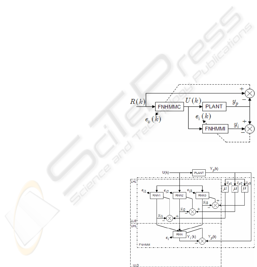
The main control objective here is to build an
inverse model of the plant in such a way that the
output of the plant tracks the system reference. It is
obvious that the control here as an open loop
feedforward learning control. The block-diagram of
this control is given on Figure 1. It contains a
FNHMM identifier (FNHMMI), which identifies the
Jacobean of the plant, and a FNHMM feedforward
controller (FNHMMC). The output of the plant and
the reference signal are normalized in the interval
[+1, -1] and divided in the same three overlapping
intervals corresponding to its membership functions
(positive, negative, and zero). The structure of the
FNHMM identifier is given on Figure 2. The local
and global errors of identification and control used
for RTNNs learning are given by the following
equations:
e
i
(k) = y
Pi
(k) - y
ii
(k); e(k) = y
p
(k) - y
i
(k) (13)
e
ci
(k) = R
i
(k) - y
Pi
(k); e
c
(k) = R(k) - y
p
(k) (14)
The FNHMMI has two levels – Lower Hierarchical
Level (LHL), and Upper Hierarchical Level (UHL).
The LHL is composed of three parts: 1)
Fuzzyfication, where the plant output signal is
divided in three intervals µ : positive [1, -0.5],
negative [-1, 0.5], and zero [-0.5, 0.5]; 2) Lower
Level Inference Engine (LLIE), which contains three
(Takagi and Sugeno, 1985) TS - fuzzy rules, given
by (10), and operating in the three intervals, and
three RTNNs, learned by the local errors of
identification (13); 3) Upper Level Defuzzyfication
(ULD) which consists of one RTNN, learned by the
global error of identification (13). This RTNN
performs a filtered weighted summation of the
outputs of the lower level RTNNs. The learning and
functioning of both levels is independent.
The block-diagram of the FNHMM feedforward
controller is given on Figure 3. During the learning,
the control errors are attenuated by the inverse of the
identified plants gain. The FNHMM feedforward
controller contains the same elements as the
FNHMM identifier. They are: fuzzyfication of the
plant output and the reference signal; lower level
inference engine, which contain the same number of
rules and RTNNs, learned by the local errors of
control (14); upper level defuzzyfication done by an
upper level RTNN, learned by the global error of
control (14).
Figure 1: Block diagram of the inverse plant model control
using FNHMM identifier and FNHMM feedforward
controller
Figure 2: Block diagram of the Fuzzy Neural Hierarchical
Multi-Model identifier
ICINCO 2005 - INTELLIGENT CONTROL SYSTEMS AND OPTIMIZATION
232
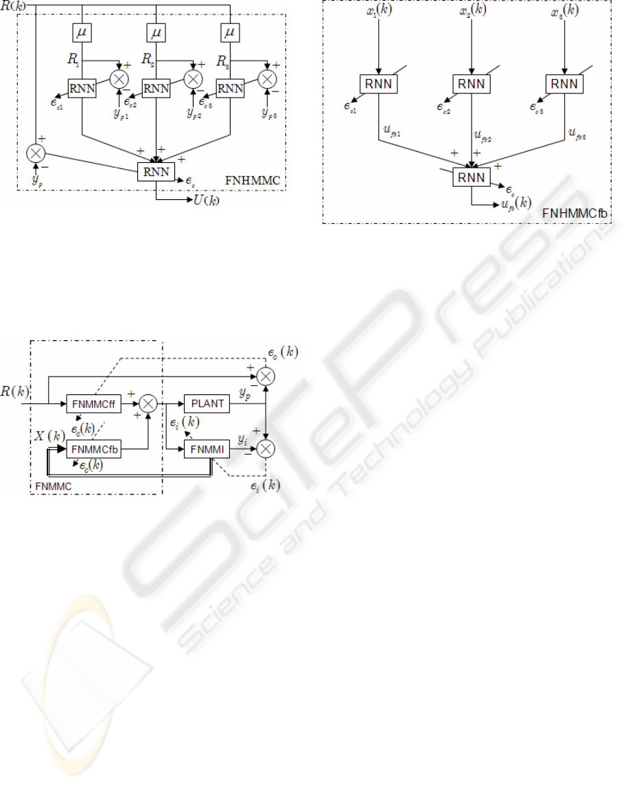
Figure 3: Block diagram of the FNHMM feedforward
controller
3.2 A Direct Adaptive FNHMM
Control Scheme
The structure of the system is given on Figure 4.
Figure 4: Block diagram of the direct adaptive neural
control scheme using FNMMI, FNMMCfb and FNMMCff
It contains a FNHMM identifier (see Figure 2),
FNHMM feedforward (see Figure 3) and feedback
(see Figure 5) controllers. The FNHMM identifier
and the FNHMM controllers contain fuzzyfier, a
Fuzzy Rule-Based System (FRBS), a set of RTNN
models and a RTNN used as defuzzyfier. The
control fuzzy rules applied and the total control,
issued by the FNMM control system are:
R
i
: If x is A
i
then u
i
= U
i
(k), i=1, 2 ,.., L (15)
U
i
(k) = - N
fb,i
[x
i
(k)] + N
ff,i
[r
i
(k)] (16)
U(k)= Σ
i
w
i
U
i
(k)
(17)
Where: r(k) is the reference signal; x(k) is the
system state; N
fb,I
[x
i
(k)] and N
ff,I
[r
i
(k)] are the
Figure 5: Block diagram of the FNMMC feedback
controller
feedforward and feedback parts of the fuzzy-neural
control, performed by RTNN functions, and w
i
are
weights, obtained from the membership functions,
corresponding to the rules (15). As it could be seen
from the equation (17), the control could be obtained
as a weighted sum of controls, given in the
consequent part of (15). In the case when the
intervals of the variables, given in the antecedent
parts of the rules, are not overlapping, the weights
obtain values one and the weighted sum (17) is
converted in a simple sum. From Figure 5 it is seen
that the FNHMM identifier approximates the plant
using three RTNNs, working in three overlapping
intervals, corresponding to the three membership
functions (positive, negative, and zero). The state
vector issued by each RTNN is entry of a feedback
FNMM controller and the FNHMM feedforward
controller complements the control part. The
defuzzification level of both control parts is
performed by RTNNs (see Figures 3 and 5).
4 SIMULATION RESULTS
Let us consider a DC-motor - driven nonlinear
mechanical system, taken from (Baruch, et al.,
2001b), which has the following friction parameters
(Lee and Kim, 1995): α = 0.001 m/s; F
s
+
= 4.2 N ;
F
s
-
= - 4.0 N; ∆F
+
= 1.8 N ; ∆F
-
= - 1.7 N ; v
cr
= 0.1
m/s; β = 0.5 Ns/m. Let us also consider that the
position and the velocity measurements are taken
with period of discretization To = 0.01 s; the system
gain is ko = 8; the mass is m = 1 kg, and the load
disturbance depends on the position and the velocity
(ld(t) = ld
1
q(t) +ld
2
v(t); ld
1
= 0.25; ld
2
= - 0.7). So
the discrete-time model of the 1-DOF mass
mechanical system is:
A HIERARCHICAL FUZZY-NEURAL MULTI-MODEL: An application for a mechanical system with friccion
identification and control
233
x
1
(k+1) = x
2
(k)
x
2
(k+1)=-0.025x
1
(k)-
0.3x
2
(k)+0.8u(k)-0.1fr(k)
(18)
v(k) = x
2
(k) - x
1
(k) (19)
y(k) = 0.1 x
1
(k) (20)
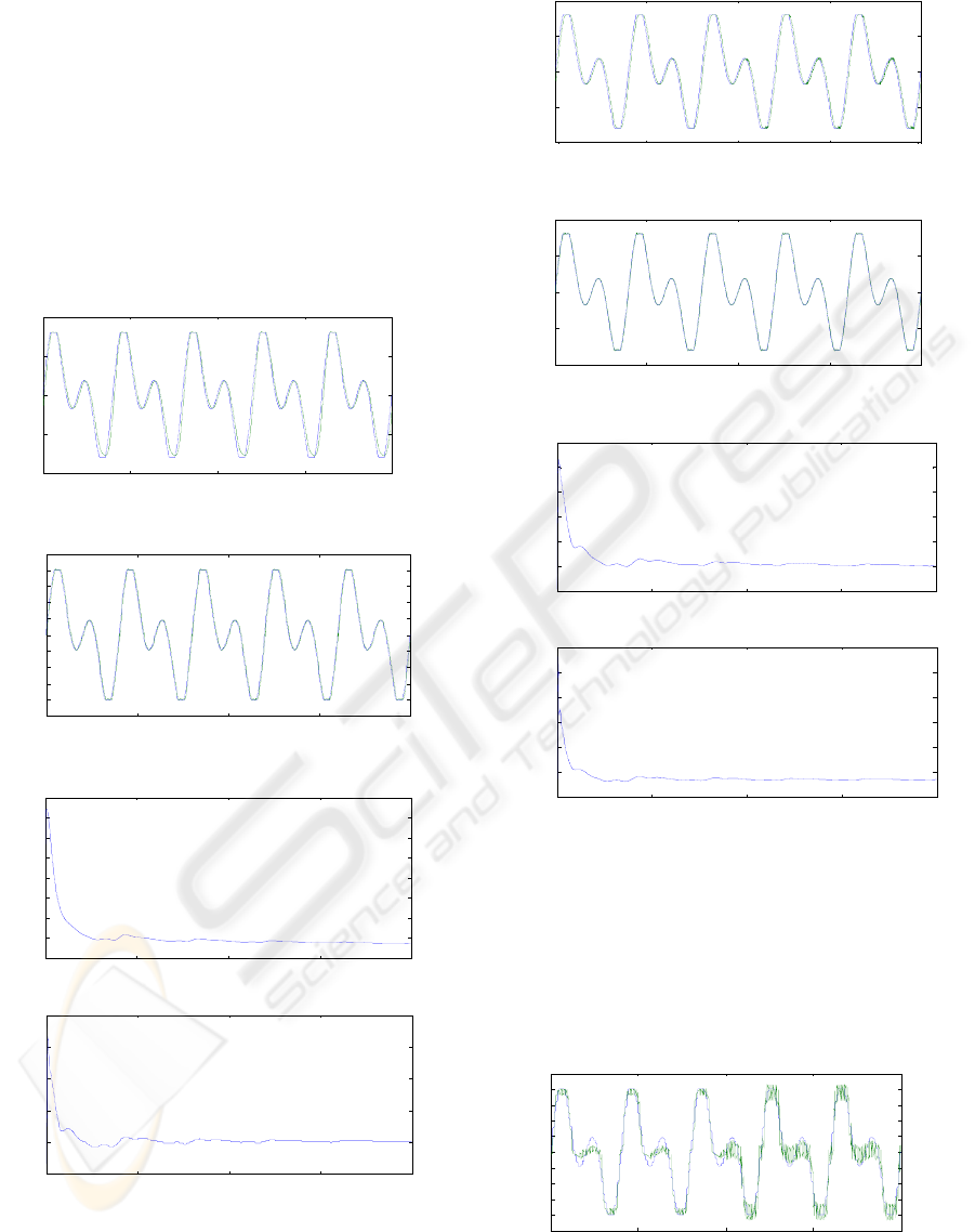
Where fr(k) is the friction force. Comparative results
of plant control for both schemes, obtained using
single RTNNs and that - using FNHMMCs, are
given on Figure 6 a,b,c,d and Figure 7 a,b,c,d. For
sake of comparison, simulation results obtained
using a fuzzy controller, are given on Figure 8 a,b.
0 5 10 15 20
-1
-0 .5
0
0.5
1
a) Comparison of the reference signal and the output of the
plant controlled by one RTNN.
0 5 10 15 20
-1
-0 .8
-0 .6
-0 .4
-0 .2
0
0.2
0.4
0.6
0.8
1
b) Comparison of the reference signal and the output of
the plant controlled by FNHMMC.
0 5 10 15 20
0
0.01
0.02
0.03
0.04
0.05
0.06
0.07
0.08
c) MSE of RTNN control.
0 5 10 15 20
0
0.5
1
1.5
2
2.5
x 1 0
-3
d) MSE of FNHMM control.
Figure 6: Trajectory tracking control results obtained with
one RTNN feedforward controller and with a feedforward
FNHMMC
0 5 10 15 20
-1
-0 .5
0
0.5
1
a) Comparison of the reference signal and the output of the
plant, using single RTNN controllers.
0 5 10 15 20
-1
-0 .5
0
0.5
1
b) Comparison of the reference signal and the output of
the plant using FNHMMC.
0 5 10 15 20
0
0.002
0.004
0.006
0.008
0.01
0.012
c) MSE of control with single RTNN controllers.
0 5 10 15 20
0
0.2
0.4
0.6
0.8
1
1.2
x 10
-3
d) MSE of control with a FNHMMC
Figure 7: Trajectory tracking control results obtained with
single RTNN feedforward/feedback control and with a
feedforward/feedback FNHMMCs
Values of the Means Squared Error of identification
and control using FNHMMs, single RTNNs, and
fuzzy control, are given on Table 1.
0 5 10 15 20
-1
-0.8
-0.6
-0.4
-0.2
0
0. 2
0. 4
0. 6
0. 8
1
a) Comparison of the reference signal and the output of the
plant.
ICINCO 2005 - INTELLIGENT CONTROL SYSTEMS AND OPTIMIZATION
234
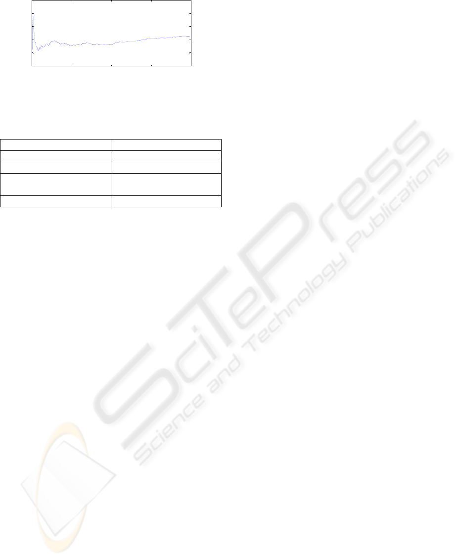
0 5 10 15 20
0
0.5
1
1.5
2
2.5
b) MSE of control.
Figure 8: Trajectory tracking control results obtained
using a fuzzy controller
Table 1: Mean Squared Error of identification and control
Name FNHMM vs. single RTNN
Systems identification: 0.08% vs. 0.27%
Feedforward control: 1.5% vs. 2.3%
Feedforward plus feedback
direct adaptive control:
0.41% vs. 2.7%
Fuzzy control: 5.8% (does not use NNs)
From Figures 6, 7, 8 and the MSE% data from Table
1, we could conclude that: the systems identification
using FNHMM gives better results than that using
only one RTNN; the control schemes which use
FNHMMC works better than that using one RTNN;
the FNHMM feedforward/feedback direct adaptive
control gives better results with respect to the
FNHMM feedforward control; the fuzzy control is
worse with respect to the neural control, especially
when the friction parameters changed.
6 CONCLUSIONS
A FNHMM for identification and control of
complex nonlinear plants is proposed. Two control
schemes of FNHMM has been experimented and
compared with a respective single-RTNN and fuzzy
control. The comparison of identification results for
a 1 DOF mechanical system with friction show that
the FNHMM identifier has a better performance
with respect to the identification using one RTNN.
The same is valid for the schemes of control. The
better control is the feedforward/feedback control
and the worse control is the fuzzy control.
REFERENCES
Babushka, R., and H. B. Verbruggen, 1997. Fuzzy
modeling: principles, methods and applications. In
Proc. of the Int. Workshop on Intelligent Control
INCON'97, Sofia, Bulgaria, Oct. 13-15, Bulgarian
Union for Automation and Informatics, pp. 1-23.
Baruch I., and E. Gortcheva, 1998. Fuzzy neural model for
nonlinear systems identification. In: Proc. of the
AARTC IFAC Workshop, Cancun, Mexico, April 15-
17, p.p. 283-288.
Baruch I., Flores J.M., Thomas F., and R. Garrido, 2001a.
Adaptive neural control of nonlinear systems. In Proc.
of the Int. Conf on NNs, ICANN 2001, Lecture Notes
in Computer Science, vol. 2130, Springer-Verlag,
Berlin, Heidelberg, N. Y., p.p. 930-936.
Baruch, I., Flores, J.M., and R. Garrido, 2001b. A fuzzy-
neural recurrent multi-model for systems identification
and control. In Proc. of the Europ. Contr. Conference,
ECC’01, Porto, Portugal, Sept. 4-7, p.p. 3540-3545.
Baruch I., Flores J.M., Nava F., Ramirez I.R., and B.
Nenkova, 2002. An advanced neural network topology
and learning, applied for identification and control of a
D.C. motor. In Proc. of the 1-st Int. IEEE Symp. on
Intelligent Syst., Varna, Bulgaria, Sept., pp. 289-295.
Eikens, B., and M.N. Karim, 1999. Process identification
with multiple neural network models. Internat.
Journal of Control, vol. 72, No 7/8, pp. 10-20.
Frasconi, P., Gori, M., and G. Soda, 1992. Local feedback
multilayered networks. Neural Computation, vol. 4,
pp. 120-130.
Gupta, M., Nikiforuk, P., and L. Jin, 1994. Adaptive
control of discrete time nonlinear systems using
recurrent neural networks. IEE Proc. Control Theory
and Applications, vol. 141, No 3, pp. 169-176.
Hunt, K.J., Sbarbaro, D., Zbikowski, R., and P. J.
Gawthrop, 1992. Neural network for control systems
(A survey). Automatica, vol. 28, pp. 1083-1112.
Hunt, K.J., Irwin, G.R., and K. Warwick, 1995. Neural
network engineering in dynamic control systems.
Springer Verlag, London.
Jin, L., and M. Gupta, 1999. Stable Dynamic
Backpropagation Learning in Recurrent Neural
Networks. IEEE Transactions on Neural Networks,
vol. 10, pp. 1321-1334.
Lee, S.W., and J.H. Kim, 1995. Robust adaptive stick-slip
friction compensation. IEEE Trans. on Ind. Elect., vol.
42 , No. 5, p.p. 474-479.
Mastorocostas P.A., and J.B. Theocharis, 2002.A recurrent
fuzzy-neural model for dynamic system identification.
IEEE Transactions on Systems, Man and Cybernetics,
Part B: Cybernetics, vol. 32, pp. 176-190.
Miller III, W.T., Sutton, R.S., and P.J. Werbos, 1992.
Neural networks for control. MIT Press, London.
Narendra K. S., and K.Parthasarathy, 1990. Identification
and control of dynamical systems using neural
networks. IEEE Transactions on Neural Networks,
vol. 1, No. 1, pp. 4-27.
Omatu, S., Khalil, M., and R. Yusof, 1995. Neuro-control
and its applications. Springer Verlag, London.
Takagi, T., and M. Sugeno, 1985. Fuzzy identification of
systems and its applications to modeling and control.
IEEE Trans. Systems, Man, and Cybernetics, vol. 15,
pp. 116-132.
A HIERARCHICAL FUZZY-NEURAL MULTI-MODEL: An application for a mechanical system with friccion
identification and control
235
