
A NEW ART GALLERY ALGORITHM FOR SENSOR
LOCATION
Andrea Bottino, Aldo Laurentini
Dipartimento di Automatica e Informatica, Politecnico di Torino, Corso Duca degli Abruzzi 24, Torino, Italy
Keywords: Art gallery, sensor positioning, planning, surveillance.
Abstract: Locating sensors in2D can be often modeled as an Art Gallery problem. Unfortunately, this problem is NP-
hard, and no finite algorithm, even exponential, is known for its solution. Algorithms able to closely
approximate the optimal solution and computationally feasible in the worst case are unlikely to exist.
However this is an important problem and algorithms with “good” performance in practical cases are sorely
needed. After reviewing the available algorithms, we propose a new sensors location incremental technique.
The technique converges toward the optimal solution. It locally refines a starting approximation provided by
an integer covering algorithm, where each edge is observed entirely by at least one sensor. A lower bound
for the number of sensor, specific of the polygon considered, is used for halting the algorithm, and a set of
rules are provided to simplify the problem.
1 INTRODUCTION
A number of computer vision tasks, as inspection,
surveillance, image based rendering, constructing
environment models, require multiple sensor
locations, or the displacement of a sensor in multiple
positions.
Sensor placement is an active area of research. A
recent survey (Scott and Roth, 1992) refers in
particular to tasks as reconstruction and inspection.
Several other tasks and techniques were considered
in the more seasoned surveys (Tarabanis et al., 1995,
Newman and Jain, 1995). Practical sensor planning
problems require considering a number of
constraints, such as image resolution, field of view
of the sensors, feature visibility, lighting, etc.
Visibility is clearly the fundamental constraint for
any kind of task and optical sensor. The sensor is
usually modeled as a point and referred to as a
“viewpoint”. A feature of an object is said to be
visible, or not occluded, from the viewpoint if any
segment joining a point of the feature and the
viewpoint does not intersects the environment or the
object itself.
Although in general the problem is three-
dimensional, in some cases it can be restricted to 2D.
This is for instance the case of buildings, which can
be modeled as objects obtained by extrusion.
For omni directional or rotating sensors, the 2D
visibility can be modeled as an Art Gallery problem,
which asks to position a minimum set of “guards” in
a polygon. Unfortunately, the problem, as well as
several of its variations, is NP-hard, and no finite
algorithm, not even exponential, for locating a
minimum set of guards is known. In addition,
algorithms computationally feasible in the worst
case and able to closely approximate the optimal
solution are unlikely to exist (Eidenbenz et al.,
2001). However, this is an important practical
problem and approximate algorithms
computationally feasible and supplying satisfactory
solutions in practical cases are sorely needed.
In this paper, after discussing the available
algorithms, we present a new approximate sensor
positioning techniques. The algorithm is incremental
and converges toward the optimal solution. It makes
use a lower bound, specific of the polygon
considered, for the number of sensors, and of rules
for locally refining a starting approximate solution.
This solution is provided by an integer covering
algorithm, where each edge must be observed
entirely by one sensor at least. The proposed
technique can also take into account constraints as
range and incidence.
242
Bottino A. and Laurentini A. (2005).
A NEW ART GALLERY ALGORITHM FOR SENSOR LOCATION.
In Proceedings of the Second International Conference on Informatics in Control, Automation and Robotics - Robotics and Automation, pages 242-249
DOI: 10.5220/0001174002420249
Copyright
c
SciTePress

2 ART GALLERY PROBLEMS
AND EDGE COVERING
The original problem, stated in 1975, refers to the
surveillance, or “cover” of polygonal areas. The
famous Art Gallery Theorem stated the upper tight
bound ⎣n/3⎦ for the minimum number of “guards”
(omni directional sensors) for covering any polygon
with n edges, metaphorically the interior of an art
gallery. The upper tight bound ⎣(n+h)/3⎦ holds for
polygons with n edges and h holes. Many variations
of the problem have been considered, and much
work has been done for finding bounds in these
cases. The decision problems related to the original
problem (are k guards sufficient for covering a given
polygon?), as well as those related to several similar
problems, has been found to be NP-hard (Danner
and Kavraki, 2002). No exact finite algorithm for
locating a minimum set of sensors is known. For
further details, the reader is referred to the
monograph of O’Rourke (1987), and to the surveys
of Shermer (1992) and Urrutia (2000).
Sensors positioning problems usually deals with
observing, or covering, the boundary of objects and
environment. Then in 2D we are content with
observing the edges of a polygonal environment. We
call this the Edge Covering (EC) problem, and the
classic problem the Interior Covering (IC) problem.
The EC problem and its relation with IC have been
analyzed in Laurentini, 1999. For both EC and IC,
the worst-case number of guards for polygons with
and without holes is the same, but an optimum set of
IC guards is not in general an optimum set of EC
guards and vice-versa, and no simple rule, as adding
or deleting guards, seems to exists for transforming
an optimal solution of one problem in an optimal
solution of the other. Also the decision problem
associated to EC is NP-hard, since the classic proofs
for polygons with and without holes also hold for
edge covering (Laurentini, 1999). As for IC, at
present no finite exact algorithm is known for
locating a minimum set of EC guards in a given
polygon.
In addition, recent result (Eidenbenz et al., 2001)
shows that no worst-case computationally feasible
approximate algorithm able to find solution close to
the optimum is likely to exist. These results apply to
both EC and IC, as well as to others problems in the
area.
Finally, let us observe that the apparently continuous
nature of EC (and IC) prevents putting the problems
in the class NP. On this point, see also O’Rourke
and Supowitz, 1983.
In the following section we will discuss the
approximate algorithms existing for EC.
3 EXISTING APPROXIMATED
EDGE COVERING
ALGORITHMS
Some approximate seasoned algorithms for IC are
reported in Shermer, 1992. All these algorithms are
polynomial. It can be easily seen that their
performance in relation with the optimal solution
can be as bad as possible (O(n) guards, where n is
the number of edges, when O(1) are sufficient).
These algorithms have not been implemented, and
no experimental results comparing the average
performances of these algorithms with the optimal
solution have been presented. Anyway, we have
seen that in general the optimal EC and IC covers
are different.
More recently, some attempt has been made for
constructing practical sensor positioning algorithms.
Kazakakis and Argyros (2002) have proposed a
heuristic that divides the polygon into a number of
convex polygons, each of which can be inspected by
a guard with visibility range restriction. The
algorithm has been implemented and some
experimental results have been reported. Time
performances are good, but the authors do not
discuss how far are the solutions from optimum.
The randomized approach (Danner and Kavraki,
2002, Gonzales-Banos and Latombe, 1998 and
2001), appears the main practical technique
available. We discuss here the most recent (not
implemented) randomized algorithm of Gonzales-
Banos and Latombe (2001), which also takes into
account range and incidence constraints. The
algorithm is as follows. First, the authors observe
that, given an optimal solution for locating the
guards, perturbing the positions of the guards into
sufficiently small areas does not affect optimality.
This leads to a randomized approach, where a
number of viewpoints are located at random in the
polygon, hoping of locating some points sufficiently
near the points of an optimal solution. The next step
consists in dividing the polygon boundaries into
cells such that each viewpoint sees exactly a set of
these cells. Selecting a minimal set of points among
the random points is equivalent to solve an NP-
complete set-covering problem. It is known that a
greedy solution is polynomial, but has an
approximation ratio bounded by (1+lgp), where p is
the cardinality of the largest subset. It is clear that
A NEW ART GALLERY ALGORITHM FOR SENSOR LOCATION
243

this factor is not a strong guarantee of good
approximation for polygons with many edges and
holes, since p is O(m(n+h)), where m is the number
of random point, which is assumed to be rather large
and in any case much larger than n. However, a
clever exploitation of the particular set structure
makes it possible to reduce the problem within an
approximation ratio of (1+ q), where q is
O(lg(n+h)
·lg(clg(n+h)) and c is the optimal size.
The advantage is that q does not depend on the
presumably large number of random points.
Concluding, the authors obtain an algorithm
polynomial in the worst-case, at the expense of the
closeness to the optimal solution. In fact, also the
improved approximation factor can be large for
polygons with hundreds of edges and some tens of
holes. In addition, it is clear that a main problem
with this algorithm is the density of the sampling, “a
choice that is perhaps more a craft than a science”
according to the authors themselves. An incremental
algorithm could be developed adding new random
points, but we have no idea of the closeness to
optimum of the solution, and we do not know where
is more convenient to add new samples.
4 WHAT AN APPROXIMATE
PRACTICAL ALGORITHM
SHOULD DO
The performance of a “good” or “practical” Art
Gallery algorithm should be analyzed in terms of
both running times and closeness to the optimal
solution of the approximation obtained. Since we
deal with a problem that we are not even able to put
in NP, we cannot be too exigent regarding the worst
case behavior, being satisfied with algorithms
capable of running in practical cases, in reasonable
times. Clearly, running time depends on the number
of edges and on the shape of the polygon. We can
assume that a reasonable choice to model many
practical environments or 2D objects is to consider
polygons with several tens, or some hundreds, of
edges. As for shape, the algorithm should be tested
with examples of real environments.
Another desirable feature of a practical algorithm is
the possibility of approaching the optimal solution
by refining an initial approximation, at the expense
of computation time. For obtaining a balanced
trade-off between precision and time, we should
have:
• some information about the quality of the
approximation obtained at each step, which
can be used to decide whether to stop the
algorithm
• an incremental algorithm, able to refine
locally the solution of the previous step.
The purpose of this paper is to present an algorithm
that, to some degree, fulfills the previous
requirements of a “good” or “practical” algorithm.
Even if we are not able to discretize an apparently
continuous problem, we propose an incremental
algorithm, able to refine locally the solution, and we
also provide a lower bound, specific of the case
considered, that can be used to decide when to stop
the incremental process. The algorithm starts with an
initial approximation supplied by an integer edge
covering algorithm.
5 INTEGER EDGE COVERING
The Integer Edge Covering (IEC) problem is a
useful restriction of EC, requiring each edge to be
entirely covered by at least one guard. For some
practical task, observing entirely a feature of an
object, usually modeled as an edge in 2D, could be
preferable. In addition, for several not particularly
tricky polygons the optimal unrestricted solution
appears not too far from an optimal integer cover.
For these reasons, integer covering is the starting
approximation of our unrestricted edge-covering
algorithm. A simple example showing the difference
between EC and IEC is shown in Fig.1
Figure 1: Two EC sensors cover the interior boundary of
the polygon, but three IEC sensors are required
Bounds for IEC have been discussed in Laurentini,
1999. Regarding complexity, it is easy to see that the
reductions of 3-SAT (O’Rourke, 1987) for polygons
with and without holes also hold for IEC, since both
reductions construct polygons where the edges are
observed entirely by at least one guard. Thus, also
the decision problem associated to IEC is NP-hard.
The difference is that the restriction allows putting
the problem in NP, so that it becomes NP-complete
and finite algorithms are possible. In fact, the
polygon can be divided into a set of non-overlapping
zones, such that each point in each zone covers
entirely the same set of edges. Then an hypothesis of
solution consists in a finite string of characters that
specifies a particular subset of these zones.
ICINCO 2005 - ROBOTICS AND AUTOMATION
244

An algorithm for finding a set of zones where
locating a minimum set of guards is reported in
Laurentini, 1999. A modified version of this
algorithm has been implemented in Bottino and
Laurentini, 2004. The algorithm works for any
polygonal environment (external coverage of
multiple polygons, internal coverage of polygons
with or without holes). Referring the readers to the
original paper for details, the main steps of the
algorithm are as follows:
IEC Algorithm
Step 1. Compute a partition Π of the viewing space
into regions Z
i
such that:
1. The same set E
i
of edges is entirely visible
from each point of Z
i
, ∀i. Actually, each
region is also labeled with the partially
visible edges and the number of occlusions.
2. The regions Z
i
are maximum regions, that is
E
i
⊄ E
j
where Z
j
is any region contiguous
to Z
i
Step 2. Select the dominant regions and the essential
regions. A region Z
i
is dominant if there is no other
region Z
j
such that E
i
⊂ E
j
. An essential zone is a
dominant zone that covers an edge not covered by
any other dominant zone.
Step 3. Find an optimum set of zones covering all
the edges. This is a set covering problem restricted
to the set of edges not covered by the essential
zones, and to the subsets corresponding to the
dominant zones that: a) are not essential; b) cover
some edge not already covered by the essential
zones.
Steps 1 and 2 are polynomial (Laurentini, 1999);
Step 3 is exponential in the worst case. However, in
many cases the simplifications introduced by
dominant and essential zones strongly reduce the
complexity of the algorithm. Observe that the
algorithm does not provide in general all the
possible minimal sets of zones, since there could be
solutions including non-dominant zones. However,
this does not seems a serious drawback, since each
non-dominant zone can be replaced by a dominant
zone that covers some more edges, and multiple
coverage in several practical cases is preferable, for
instance in case of sensor failure.
6 THE SENSOR POSITIONING
ALGORITHM
Integer edge covering provides a starting
approximation, which can be incrementally refined
for approaching the optimal unrestricted solution.
For deciding if a solution is acceptable, we compute
a lower bound LB(P) for the optimum number of
sensors, specific of the polygon P considered. If the
starting solution is far from the lower bound, we can
improve this solution by splitting some of the edges
and re-applying the IEC algorithm. It is clear that
this procedure converges toward the optimal
solution, if computationally feasible. For reducing
the computational burden, we also supply rules that
tell us which edges must not be divided in order to
reach the optimal solution. Summarizing, our sensor
positioning algorithm works as follows.
Given a polygon P, compute the lower bound LB(P)
with the LBA algorithm described in section 6.2
Apply the IEC algorithm and find an approximate
covering. Compare the cardinality CA of the
approximate covering with the lower bound. If they
are equal, the solution is optimal also for the
unrestricted problem. If (CA/LB(P))<1+ε, where ε is
some predefined threshold, stop; otherwise:
Apply the algorithm INDIVA, described in section
6.3 for finding the edges that must not be divided,
split the others and return to 2
Actually, it could be necessary to stop the
algorithm before reaching a satisfactory cover due to
the computation time. In the rest of this section we
describe the algorithms INDIVA and LBA.
6.1 Integer and weak visibility
polygons
Both algorithms LBA and INDIVA make use of the
concept of weak and integer visibility polygons of
the edges (J. O'Rourke, 2002). Let us briefly recall
their definitions:
the Weak visibility polygon W(e
i
) of an edge e
i
is the
polygon whose points see some points of e
i
the Integer visibility polygon I(e
i
) is the polygon
whose points see entirely e
i.
An example is shown in
Fig.2
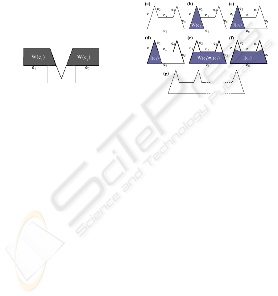
Figure 2: The integer and weak visibility polygons of the
edge e
Polynomial algorithms for computing weak and
integer visibility polygons of an edge are described
in the literature (Sack and Suri, 1990). In our case
however, both polygons can be computed as a
byproduct of the IEC algorithm. If there are p zones
A NEW ART GALLERY ALGORITHM FOR SENSOR LOCATION
245
in the partition Π, computing the visibility polygons
for all edges is O(pn).
6.2 LBA, the Algorithm for Finding
a Lower Bound
LBA Algorithm finds a maximum subset of disjoint
(not intersecting) weak visibility polygons W(e
i
).
The cardinality of this set is LB(P).
Since each weak visibility polygon must contain at
least one sensor, no arrangement of EC sensors can
have fewer sensors than LB(P). A simple example is
shown in Fig.3, where the lower bound is 2.
Figure 3: A maximum set of non-intersecting weak
visibility polygons
Computing the lower bound requires solving the
maximum independent set problem for a graph G
where each node represents the weak visibility
polygon of an edge of P, and each edge of G
connects nodes corresponding to intersecting weak
visibility polygons. The problem is equivalent to the
maximum clique problem for the complement graph
G’ (the graph obtained by joining those pairs of
vertices that are not adjacent in G). It is well known
that these are NP-complete problems.
However, we stress that exact branch-and-bound
algorithms for these problems have been presented
and extensively tested (Woods, 1997, Oestergard,
2002), showing more than acceptable performance
for graphs with hundreds of nodes. Then, we assume
that computing LB(P) is computationally feasible for
the practical cases considered.
6.3 INDIVA, the Algorithm for
Finding Indivisible Edges
In this section we describe a set of rules for finding
the indivisible edges of P. An edge is called
indivisible if optimal sets of sensors exist such that
edge is entirely observed by at least one sensor.
Clearly, for approaching these optimal solutions we
do not need to split these edges. The first two rules
are as follows:
Rule1. If W(e
i
) = I(e
i
), e
i
is indivisible.
Rule2. If W(e
i
) ⊆ I(e
j
), e
j
is indivisible.
Both rules follows from the fact that at least one
sensor of any minimum set must be located in each
weak visibility polygon, and then also in the integer
visibility polygon satisfying one of the above rules.
A simple example will show how to apply these
rules, and that they can be powerful tools for
simplifying the problem. Let us consider the
polygon in fig. 2(a).
Figure 4: In this case, the optimum EC and IEC covers are
equal
The weak visibility polygon of e
2
is shown in (b). It
is coincident (c) with the integer visibility polygon
I(e
2
), and then for Rule 1 e
2
is indivisible, and
marked with a thicker line. In (d) it shown that I(e
1
)=
W(e
2
), and then for Rule 2 also e
1
is indivisible, as
well as, for similar reasons, e
4
and e
5
. As for e
3
, it is
indivisible, since W(e
3
)= I(e
3
) (Fig.1 (e). Finally, in
(f) it is shown I(e
6
). Since I(e
6
)⊃W(e
3
), also e
6
is
indivisible.
Concluding, in this example the unrestricted
minimal set of guards is that provided by the integer-
covering algorithm. The same result could have been
obtained by computing the IEC solution, whose
cardinality is equal to the lower bound LB(P). This
also happens for any polygon of the family shown in
(g), which is used for showing that the bound
supplied by the Art Gallery theorem is tight.
We stress that if one of previous rules can be applied
to an edge, this edge is entirely observed by a sensor
for any optimal solution.
We have found three other rules for determining
other edges indivisible for some optimal solution.
They are based on the idea that for some edge e we
can discard some parts of W(e), having lesser
visibility of the boundary of P than other parts.
Let us recall that the algorithm IEC divides P into a
set of regions whose points share the same visibility
condition of the boundary of P. In particular, each
zone is labeled with: a) the edges seen entirely by
each point of the region; b) the edges seen partially
ICINCO 2005 - ROBOTICS AND AUTOMATION
246
with the number of occlusions. Let E(p) denote the
points of the boundary of P seen by a point p,
excluding points belonging to indivisible edges,
which are fully observed by some other viewpoint.
We say that a region R of W(e
i
) is the best region of
W(e
i
) if for any point p∈R and any point q∈(
W(e
i
)- R) it is E(p)⊇ E(q). It is clear that, if such
region exists, any optimal solution with one
viewpoint in W(e
i
)-R can be substituted by an
optimal solution with a viewpoint in R. It follows
that all the edges fully observed by R are indivisible.
Then we get the following rule:
Rule3: edges which are completely seen by any
point belonging to the best region of W(e) (if it
exists) are indivisible.
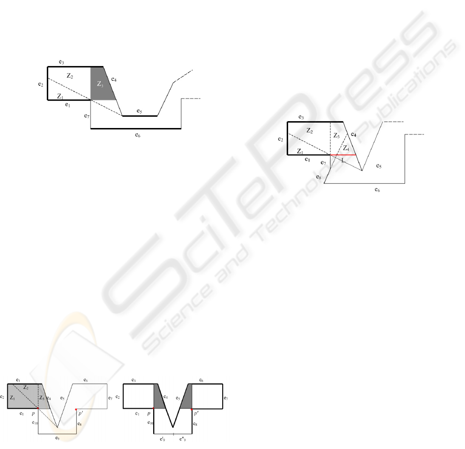
Figure 5: Z
3
is the best region of W(e
1
)
As an example, consider the polygon of Fig. 5. By
applying Rules 1) and 2) we find that edges e
1
, e
2
, e
3
,
e
5
, e
6
are indivisible. Consider W(e
1
). Region Z
1
sees
fully edges e
1
, e
2
, e
3
and partially e
4
. Region Z
2
sees
fully edges e
1
, e
2
, e
3,
e
4
and partially e
6
, which must
not be considered since it has been already found to
be indivisible. Then Z
3
is the best region, since any
point in it sees fully edges e
1
, e
2
, e
3
, e
4
and e
7
.
Concluding, we have found that also e
4
and e
7
are
indivisible.
The best point of W(e) is defined (if it exist) as the
point p
o
of W(e) such that E(p
o
)⊇E(q) (excluding
indivisible edges) for any other point q∈W(e
i
). If
such a point exists, in any optimal solution a
viewpoint belonging to W(e
i
) can be substituted by
p
o
. Then we get the following rule:
Rule 4: An edge is indivisible if it is observed by the
best point of W(e)
Consider the example of Fig.6.
(a) (b)
Figure 6: Point p is the best point of W(e
1
) (a). The zones
where two optimal viewpoints can be located (b)
We assume that a viewpoint lying on a vertex of P is
able to see the edges converging at the vertex. This
is justified by the fact that, excluding exceptional
alignment conditions, p can be displaced in a region
nearby without affecting the optimality. Using rules
1 and 2 e
1
, e
2
, e
3
are easily found to be indivisible. It
is clear that p, which sees entirely e
1
, e
2
, e
3,
e
4
, e
10
,
and a part of e
9
largest or equal to that seen by any
other point is the best point of W(e
1
). Then also e
4
and e
10
are indivisible.
The full algorithm for this polygon works as follows.
LB(P) is 2, as shown in Fig.3. Applying the IC
algorithm we obtain 3 viewpoints. Since this is
different from the lower bound, we apply rules 1, 2
and 4 and find that only e
9
could be divided. After
splitting in two e
9
we apply again the IC algorithm,
and find two areas, containing the two best points p
and p’ where the viewpoints can be independently
located (Fig. 6(b)). The cardinality of the solution is
equal to LB(P), and then the solution is optimal.
Figure 7: The line L contains the best boundary points
Let us observe that the definition of best point of a
region W(e
i
) can be extended, excluding from E(p)
not only other indivisible edges, but also edges or
parts of edges covered by other best points. This is
an effective extension, as it will be shown by the
second example in section 7.
Finally, consider W(e
1
) in the case shown in Fig.7.
Applying rules (1) and (2) we find that e
1
, e
2
, e
3
are
indivisible. However, we are not able to apply rules
(3) or (4), since in W(e
1
) there is no best point or
region according to the definition given. This
depends on the fact that there is no point or region
that sees a part of e
6
larger then any other point.
However, we observe that, for each point p∈W(e
1
),
there is a point of the boundary line L that sees the
same set of integer edges, and a larger part of e
6
.
This means that any minimal solution with a
viewpoint point inside W(e
1
) can be transformed in a
minimal solution with a viewpoint lying on L. In
these minimal solution the set of edges entirely
observed is the set entirely observed by any point of
L, in this case e
1
, e
2
, e
3
, e
4
, e
7
. Then also e
4
and e
7
are
indivisible. We will call a line L the best boundary
lines of W(e) if, for any point q∈W(e) there is a
point p∈L such that E(p)⊇ E(q). We obtain:
A NEW ART GALLERY ALGORITHM FOR SENSOR LOCATION
247
Rule 5: An edge is indivisible if it is entirely
observed by any point of the best boundary line (if it
exists)
7 TWO EXAMPLES
First, let us apply our algorithm to a polygon taken
from the paper (Gonzales-Banos and Latombe,
2001) of Danner and Kavraki.
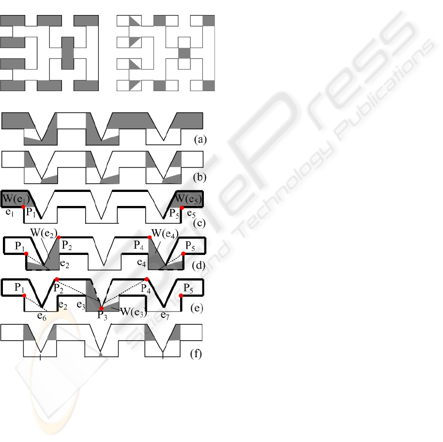
Figure 8: LB(P) (left) and an optimal solution (right)
Figure 9: In this case, the algorithm reaches in a few steps
the optimal solution
The cardinality of the maximum set of non-
intersecting weak visibility regions (shown on the
left in Fig.8) is 9. Then LB(P) = 9.
One of the minimum solutions provided by the IC
algorithm is shown in Fig 8 on the right. Since the
number of zones where to independently locate a
minimum set of integer edge guards is 9, this is also
an optimal solution of the unrestricted problem.
In the second example (Fig.9), LB(P) is 5 (Fig.9(a)
and the cardinality of the IC approximation is 7(in
Fig.7(b) one optimal integer cover is shown). Rules
(1), (2) and (4) determine the indivisible edges
shown in Fig.9(c), and two best points of W(e
1
) and
W(e
5
). Applying again rule (4) taking into account
the edges and parts of edges (hatched in the figure)
observed by the two best points, two other best
points of W(e
2
) and W(e
4
) are found(Fig. 9(d)).
Another application of rule (4) supplies the best
point of W(e
5
) (Fig.9(e)). Concluding, all edges are
indivisible, excluding e
6
and e
7
. Splitting in two
these edges and applying again the IEC algorithm,
the solution shown in Fig.9(f) is found. Five sensors
can be located anywhere in the five regions shown,
and therefore solution is optimal.
8 CONCLUSIONS AND FUTURE
WORK
We have presented a new art gallery sensor location
algorithms. The algorithm starts with an
approximate solution provided by an integer edge
covering algorithm, since in many practical cases
this appears not too far from the optimal solution. A
lower bound for the optimal number of sensor is
computed. If the cardinality of the solution is equal
to the lower bound, the solution is optimal; if not, an
optimal solution can be approached by a local
refinement of the integer edge covering solution. A
set of rules is provided for determining which edges
could be split to approach the optimal solution.
Some examples show how the algorithm works.
Is the algorithm a “good” algorithm for practical
cases, or, in other words, does it supplies in
reasonable time’s solutions close to the optimum?
For assessing its performance, we are currently
implementing the full algorithm and looking for
further rules for finding indivisible edges, as well as
rules for splitting divisible edges. Then we will
apply the algorithm to a number of 2D maps taken
from real environments.
A final remark. Our algorithm can easily take into
account range and incidence constraints. For each
edge e the constraints define a region C(e) of P
where the viewpoint can be located. Applying the
IEC algorithm, we must consider as candidates to
cover an edge e only the regions, or their parts,
belonging to C(e).
ICINCO 2005 - ROBOTICS AND AUTOMATION
248

REFERENCES
A. Bottino, A. Laurentini "Optimal positioning of sensors
in 2D". Proc. 9th Iberoamerican Congress on Pattern
Recognition, Puebla (Mexico), October 26-29, 2004
J.C. Culberson and R.A. Reckhow,” Covering polygons is
hard,” J Algorithms , Vol.17, pp. 2–44,1994
T. Danner and L.E. Kavraki,” Randomized planning for
short inspections paths,” IEEE Int. Conf. On Robotics
and Automation,April 2002, pp. 971-976
S.Eidenbenz, C. Stamm and P. Widmayer,“
Inapproximability results for guarding polygons and
terrains,” Algorithmica, Vol.31, pp.79-113, 2001
H. Gonzales-Banos and J-C. Latombe,” A randomised art
gallery algorithm for sensor placement,” ACM
SCG’01, June3-5,2001
H. Gonzales-Banos and J-C. Latombe.”Planning robot
motion for range-image acquisition and automatic 3D
model construction,” Proc. AAAI Fall Symposyum
Series, 1998
G. D. Kazakakis, and A.A. Argyros, “Fast positioning of
limited visibility guards for inspection of 2D
workspaces,” Proc. 2002 IEEE/RSJ Intl. Conf. On
Intelligent Robots and Systems, pp.2843-2848,
October 2002
A.Laurentini,”Guarding the walls of an art gallery,” The
Visual Computer, vol.15, pp.265-278, 1999
T.S. Newman and A.K. Jain, “A survay of automated
visual inspection,” Comput. Vis. Image Understand. ,
vol.61, no.2, pp.231-262, 1995
J. O’Rourke and K.J. Supowit, “Some NP-hard polygon
decomposition problems,”IEEE Trans IT, Vol.29,
no.2, pp.181-190, March 1983
J. O'Rourke , Art gallery theorems and algorithms, Oxford
University Press, New York,1987
P. Oestergard, “A fast algorithm for the maximum clique
problem,”Discrete Applied Mathematics,Vol.120,
pp.197-207, 2002
J.R.Sack and S.Suri,”An optimal algorithm for detecting
weak visibility of a polygon,” IEEE Trans. on
Computers,Vol.39, pp.1213-1219, 1990
T. Shermer, “Recent results in art galleries,” IEEE Proc.
Vol. 80, pp.1384-1399, 1992
W.R.Scott and G.Roth,”View planning for Automated
Three-Dimensional Object Reconstruction and
Inspection,” ACM Comput. Surveys,Vol.35, No.1,
March 2003, pp.64-96
K.A. Tarabanis, P.K. Allen, and R. Y. Tsai, “ A survey of
sensor planning in computer vision,” ,” IEEE Trans.
Robot. and Automat., vol. 11, no. 1 , pp. 86 –104,
1995
J. Urrutia, "Art Gallery and Illumination Problems"
Handbook on Computational Geometry, Elsevier
Science Publishers, J.R. Sack and J. Urrutia eds. pp.
973-1026, 2000.
D.R. Woods,” An algorithm for finding a maximum clique
in a graph,” Operations Research Letters,
Vol.21, pp.
211-217,1997
A NEW ART GALLERY ALGORITHM FOR SENSOR LOCATION
249
