
TRACKING OF A UNICYCLE-TYPE MOBILE ROBOT USING
INTEGRAL SLIDING MODE CONTROL
Michael Defoort, Thierry Floquet and Wifrid Perruquetti
LAGIS UMR CNRS 8146, Ecole Centrale de Lille
BP 48, Cite Scientifique, 59 651 Villeneuve-d’Ascq, France
Annemarie Kokosy
LAGIS UMR CNRS 8146, ISEN
41 bvd Vauban, 59 046 Lille Cedex, France
Keywords:
Nonholonomic mobile robot, sliding mode, tracking control, unmatched uncertainty.
Abstract:
This paper deals with the tracking control for a dynamic model of a wheeled mobile robot in the presence of
some perturbations. The control strategy is based on integral sliding mode. Simulations illustrate the results
on the studied mobile robot.
1 INTRODUCTION
One of the motivations for tackling the tracking
of nonholonomic systems is the large number of
applications mobile robots (Laumond, 1998). One
difficulty for motion planning and control of a
car-like robot arises from the so-called nonholonomic
constraints imposed by the rolling wheels.
Obstacles to the tracking of such systems are the
uncontrollability of their linear approximation and
the fact that the Brockett’s necessary condition
to the existence of a smooth time-invariant state
feedback is not satisfied (Brockett, 1983). To
overcome those difficulties, various methods have
been investigated: homogeneous and time-varying
feedbacks (Pomet, 1992; Samson, 1995), sinu-
soidal and polynomial controls (Murray and Sastry,
1993), piecewise controls (Hespanha and Morse,
1999; Monaco and Normand-Cyrot, 1992), flatness
(Fliess et al., 1995), backstepping approaches (Jiang,
2000) or discontinuous controls (Floquet et al., 2003).
In this paper, it is aimed to design a control law for
the unicycle-type mobile robot which:
• solves the disturbance rejection problem for
bounded matching perturbations and some un-
matched disturbance from the initial time instance,
• is a good compromise between performance and
robustness,
• takes into account the actuator dynamics.
This objective will be achieved by using integral
sliding mode control law. Sliding mode control
(Edwards and Spurgeon, 1998) is a powerful method
to control nonlinear dynamic systems operating
under uncertainty conditions. A drawback of such a
control is that the trajectory of the designed solution
is not robust on a time interval preceding the sliding
motion. In (Utkin and Shi, 1996; Poznyak et al.,
2004; Cao and Xu, 2004), a new sliding mode
design concept, namely integral sliding mode (ISM),
without any reaching phase was proposed. Thus, the
robustness can be guaranteed throughout an entire
response of the system starting from the initial time
instance.
Here, the proposed controller is based on the integral
sliding mode in order to solve the tracking problem
in presence of matching and some unmatching
perturbations.
The outline of this paper is as follows. Section II
formulates the tracking problem. Then, the use of in-
tegral sliding mode, in section III, enables to solve the
problem of tracking the reference trajectory in spite of
perturbations. Finally, in section IV, numerical exam-
ples illustrate the effectiveness of the proposed con-
troller.
2 PROBLEM STATEMENT
In this paper, we consider the unicycle-type robot
which behavior can be described by the following sys-
106
Defoort M., Floquet T., Perruquetti W. and Kokosy A. (2005).
TRACKING OF A UNICYCLE-TYPE MOBILE ROBOT USING INTEGRAL SLIDING MODE CONTROL.
In Proceedings of the Second International Conference on Informatics in Control, Automation and Robotics - Robotics and Automation, pages 106-111
DOI: 10.5220/0001173501060111
Copyright
c
SciTePress

tem (see (de Wit and Sordalen, 1992) for details):
⎧
⎨
⎩
˙x = u cos(θ)+p
1
(X)
˙y = u sin(θ)+p
2
(X)
˙
θ = v + p
3
(X)
, (1)
where X =[x, y, θ] is the state, x and y are the coor-
dinates of the center gravity of the robot, θ is the ori-
entation of the car with respect to the x-axis. p
1
(X),
p
2
(X) and p
3
(X) are some additive perturbations due
to parameter variations, unmodeled dynamics or ex-
ternal disturbances assumed to be smooth enough and
thus bounded over some compact set. u and v refer
respectively to the applied linear and the angular ve-
locities (see Fig. 1).
Figure 1: Unicycle robot kinematic
Discontinuous control laws have been developed in
the literature in order to stabilize system (1) (Astolfi,
1996; Floquet et al., 2003). The main criticism when
applying such strategies to a mobile robot would be
the action of a discontinuous control directly on the
mechanical part of the system (namely u and v). The
purpose of the paper is to define a sliding mode con-
trol acting on the electrical parts of the system (which
is more realistic since power converters are discontin-
uous actuators by nature). Taking into account the ac-
tuator dynamics remains to include some dynamical
extensions (cascaded integrators) in the system (1):
⎧
⎪
⎪
⎪
⎪
⎪
⎨
⎪
⎪
⎪
⎪
⎪
⎩
˙x = u cos θ + π
1
˙y = u sin θ + π
2
˙
θ = v + π
3
˙u =
F
m
− α
1
u + π
4
˙v =
τ
J
− α
2
v + π
5
˙
F = P + π
6
, (2)
where m is the mass, J is the inertia, α
1
, α
2
are pos-
itive scalars coming from the actuator dynamics, F
is the force, X =[x, y, θ, u, v, F ]
T
and U =[P, τ]
T
are respectively the new state and the control input.
π =[π
1
,...,π
6
]
T
is an additive perturbation (π
1
, π
2
,
π
3
and π
4
are sufficiently smooth function of time).
Assume that the desired, feasible trajectory X
r
=
[x
r
,y
r
,θ
r
,u
r
,v
r
,F
r
]
T
satisfies the following dy-
namics where U
r
=[P
r
,τ
r
]
T
is the reference input.
⎧
⎪
⎪
⎪
⎪
⎪
⎨
⎪
⎪
⎪
⎪
⎪
⎩
˙x
r
= u
r
cos θ
r
˙y
r
= u
r
sin θ
r
˙
θ
r
= v
r
˙u
r
=
F
r
m
− α
1
u
r
˙v
r
=
τ
r
J
− α
2
v
r
˙
F
r
= P
r
. (3)
The output tracking error is denoted by:
e =[e
1
,e
2
]
T
=[x − x
r
,y− y
r
]
T
. (4)
Our control purpose is to design an appropriate
controller such that the vehicle (2) is forced to
asymptotically track the desired trajectory (3) from
some initial tracking errors in spite of the perturba-
tions. In fact, the goal is to asymptotically stabilize
the tracking errors e
1
and e
2
and their time derivatives
to zero.
3 CONTROLLER DESIGN FOR
TRAJECTORY TRACKING
Sliding mode control, which consists in constraining
the motion of the system along manifolds of reduced
dimensionality in the state space, is quite popular in
nonlinear control systems community. One can refer
to (Perruquetti and Barbot, 2002) for further details
about this theory. Its robustness properties with re-
spect to matching perturbations and its discontinuous
character also motivated the authors to consider such
an approach for the tracking of the nonholonomic
system (2).
Let us differentiate the tracking errors e once with
respect to time:
˙e =
u cos θ − ˙x
r
u sin θ − ˙y
r
+
π
1
π
2
(5)
Since neither P nor τ appears in (5), one can differ-
entiate further with respect to time until they appear:
¨e =
⎡
⎢
⎢
⎢
⎣
(
F
m
− α
1
u)cosθ
−uv sin θ − ¨x
r
(
F
m
− α
1
u)sinθ
+uv cos θ − ¨y
r
⎤
⎥
⎥
⎥
⎦
+
⎡
⎢
⎢
⎢
⎣
˙π
1
+ π
4
cos θ
−uπ
3
sin θ
˙π
2
+ π
4
sin θ
+uπ
3
cos θ
⎤
⎥
⎥
⎥
⎦
(6)
and
e
(3)
= ξ(X)
P
τ
+
φ
1
(X)
φ
2
(X)
+
K
1,3
(X)
K
2,3
(X)
(7)
TRACKING OF A UNICYCLE-TYPE MOBILE ROBOT USING INTEGRAL SLIDING MODE CONTROL
107

with
ξ(X)=
cos θ
m
−
u sin θ
J
sin θ
m
u cos θ
m
,
φ
1
(X)
φ
2
(X)
=
⎡
⎢
⎢
⎢
⎢
⎢
⎢
⎢
⎢
⎣
−x
(3)
r
− α
1
(
F
m
− α
1
u)cosθ
−2v(
F
m
− α
1
u)sinθ
+uα
2
v sin θ − uv
2
cos θ
−y
(3)
r
− α
1
(
F
m
− α
1
u)sinθ
+2v(
F
m
− α
1
u)cosθ
−uα
2
v cos θ − uv
2
sin θ
⎤
⎥
⎥
⎥
⎥
⎥
⎥
⎥
⎥
⎦
,
K
1,3
(X)
K
2,3
(X)
=
⎡
⎢
⎢
⎢
⎢
⎢
⎢
⎢
⎢
⎢
⎢
⎢
⎣
(−α
1
π
4
+˙π
4
)cosθ − 2vπ
4
sin θ
−2π
3
(
F
m
− α
1
u + π
4
)sinθ
−u(π
5
+˙π
3
)sinθ − 2uvπ
3
cos θ
(π
6
− uπ
3
2
)cosθ+¨π
1
(−α
1
π
4
+˙π
4
)sinθ +2vπ
4
cos θ
+2π
3
(
F
m
− α
1
u + π
4
)cosθ
+u(π
5
+˙π
3
)cosθ − 2uvπ
3
sin θ
(π
6
− uπ
3
2
)sinθ+¨π
2
⎤
⎥
⎥
⎥
⎥
⎥
⎥
⎥
⎥
⎥
⎥
⎥
⎦
.
The decoupling matrix is ξ(X) and
det(ξ(X)) =
u
Jm
.
So, a singularity appears at u =0. Therefore, the
linear velocity must be ensured to be different from
zero.
From (7), let us design
u
1
u
2
= ξ(X)
P
τ
+
φ
1
(X)
φ
2
(X)
(8)
From (5), (6), (7) and (8), two linear sub-systems
are obtained, for i ∈{1, 2}:
⎡
⎣
˙e
i
¨e
i
e
(3)
i
⎤
⎦
=
010
001
000
e
i
˙e
i
¨e
i
+
0
0
1
u
i
+
K
i,1
K
i,2
K
i,3
(9)
where K
i
=[K
i,1
,K
i,2
,K
i,3
]
T
are external distur-
bances resulting from (5), (6) and (7):
K
1,1
K
2,1
=
π
1
π
2
,
K
1,2
K
2,2
=
˙π
1
+ π
4
cos θ − uπ
3
sin θ
˙π
2
+ π
4
sin θ + uπ
3
cos θ
.
Using E
i
=[e
i
, ˙e
i
, ¨e
i
]
T
, system (9) can be des-
cribed in a compact form:
˙
E
i
= AE
i
+ Bu
i
+ K
i
, (10)
The perturbations K
i
, i ∈{1, 2}, are split as fol-
lows:
K
i
= h
i
+ k
i
where h
i
is smooth uncertainty representing the
perturbations which satisfy the so called ”standard
matching condition”, that is to say h
i
∈ span(B),
i.e. h
i
= Bq
i
and k
i
represents the unmatched part.
Assumption: q
i
and k
i
are bounded by known non-
linear functions as follows:
q
i
≤
i
(E
i
),
k
i
≤ρ
i
(E
i
).
For system (10), the control law is defined as fol-
lows
u
i
= u
i,0
+ u
i,1
. (11)
where u
i,0
is the ideal control and u
i,1
represents the
ISM part which will be designed to be discontinuous
in order to reject the perturbation.
The first part of the control design is to find a con-
trol law u
i,0
such that the ideal closed-loop system
˙
E
i
= AE
i
+ Bu
i,0
is globally asymptotically stable.
The following control enables to stabilize the tracking
errors:
u
i,0
= −β
i
E
i
,β
i
=[β
i,1
,β
i,2
,β
i,3
] (12)
The constant real coefficients {β
i,1
,β
i,2
,β
i,3
} are
chosen appropriately such that the ideal system is
globally stable.
However, with the control law (12), the system
is not robust with respect to the perturbations K
i
(see Section 4, Fig. 3). So, to this first controller,
a discontinuous term is added based on ISM to en-
sure the desired performance despite the disturbances.
Define the sliding function σ
i
as:
σ
i
= σ
i,0
+ z
i
(13)
The first term σ
i,0
is a linear sliding surface designed
as follows:
σ
i,0
= D
i
E
i
where D
i
∈ R
1×3
is constant and is selected such
that the matrix D
i
B is nonsingular (for instance,
D
i
= B
+
=[0, 0, 1] where B
+
is the pseudo-inverse
of B).
The second term z induces the integral term. The
main idea of ISM (Utkin and Shi, 1996) is to elim-
inate the reaching phase by enforcing sliding mode
throughout the entire system response. To achieve the
stabilization of system (10), the equivalent control of
ICINCO 2005 - ROBOTICS AND AUTOMATION
108

u
i,1
(denoted u
i,1eq
), which describes the system tra-
jectory when sliding mode takes place in (13), should
fulfill:
u
i,1eq
= −q
i
− [D
i
B]
−1
D
i
k
i
. (14)
Furthermore, in sliding mode, along the system tra-
jectories, one should have:
˙σ
i
= D
i
˙
E
i
+˙z
i
= D
i
(AE
i
+ Bu
i
+ K
i
)+ ˙z
i
= D
i
(AE
i
+ Bu
i,0
+ Bq
i
+ k
i
)
+D
i
Bu
i,1
+˙z
i
=0
(15)
Conditions (14) and (15) holds if:
˙z
i
= −D
i
(AE
i
+ Bu
i,0
)
z
i
(0) = −σ
i,0
(0) (16)
That is to say:
z
i
= −D
i
E
i
(0) −
t
0
(D
i
(AE
i
+ Bu
i,0
))ds
where the initial condition z(0) is determined from
σ
i
(0) = 0. Hence, the sliding mode occurs from the
initial time instance.
The control u
i,1
in (11) is defined to enforce sliding
mode along the manifold (13) and is of the following
form:
u
i,1
= −M
i
(E
i
) sign (D
i
Bσ
i
) (17)
where the switching gain satisfies
M
i
(E
i
) >
i
(E
i
)+[D
i
B]
−1
D
i
ρ
i
(E
i
). (18)
Proposition: The controller defined in (11), (12),
(17) solves the tracking problem if the unmatched per-
turbation satisfy, for i =1, 2:
I − B[D
i
B]
−1
D
i
ρ
i
(E
i
) <λ
i,min
E
i
(19)
where λ
i,min
is the lowest eigenvalue of the matrix
A − Bβ
i
.
Proof: Let us choose the following Lyapunov func-
tion
V
i
=
1
2
σ
2
i
From the choice of the switching gain (18), the time
derivative of this function can be expressed as:
˙
V
i
= σ
i
(D
i
(AE
i
+ Bu
i
+ h
i
+ k
i
)
−D
i
(AE
i
+ Bu
i,0
))
= σ
i
D
i
(Bu
i,1
+ Bq
i
+ k
i
)
= σ
i
D
i
B(u
i,1
+ q
i
+[D
i
B]
−1
D
i
k
i
)
≤−η
i
|D
i
Bσ
i
|,η
i
∈ R
+∗
≤ 0
Thus, the trajectory evolves on the manifold σ
i
=0
from t =0and remains there in spite of the perturba-
tions.
Since, in sliding mode, (14) is satisfied, the closed
loop dynamics becomes:
˙
E
s
i
= AE
s
i
+ Bu
i,0
+ {I − B[D
i
B]
−1
D
i
}k
i
where the subscript s denotes the state vector in
sliding mode.
Choosing a Lyapunov function as
V
s
=
2
i=1
(E
s
i
)
T
E
s
i
2
,
one gets,
˙
V
s
=
2
i=1
(E
s
i
)
T
(AE
s
i
+ Bu
i,0
)
+
2
i=1
(E
s
i
)
T
(I − B[D
i
B]
−1
D
i
)k
i
≤−
2
i=1
λ
i,min
E
s
i
2
+
2
i=1
E
s
i
I − B[D
i
B]
−1
D
i
ρ
i
According to (Qu, 1998), the tracking errors is
globally asymptotically stable if the unmatched
perturbation satisfy (19).
Remark: As the system (2) without perturbation
(π
1
and π
2
are supposed to be vanishing) is flat (Fliess
et al., 1995), the tracking errors in orientation will
converge to zero. Indeed,
θ − θ
r
= atan
˙y
˙x
− atan
˙y
r
˙x
r
tends to zero when ˙x → ˙x
r
and ˙y → ˙y
r
.
4 SIMULATION RESULTS
4.1 Tracking problem
In this simulation, the desired trajectory is circular.
The mobile robot is required to track, from an initial
point X(0), the circular trajectory:
x
r
(t)=R cos(at)
y
r
(t)=R sin(at)
TRACKING OF A UNICYCLE-TYPE MOBILE ROBOT USING INTEGRAL SLIDING MODE CONTROL
109
with R =20and a =0.01π which is represented by
the dashed line in the following figures. The reference
orientation can be deduced from ˙x
r
and ˙y
r
, i.e.
˙
θ
r
= a.
The initial state X(0) for the vehicle is:
x(0) = 22,y(0) = −1,θ(0) =
π
2
+0.01,
u(0) = 0.2,v(0) = 0,F(0) = 0.
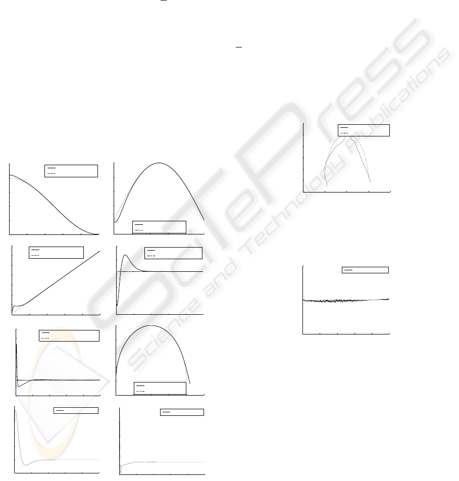
4.1.1 Simulation without uncertainties
Using the control inputs defined in (12), the tracking
errors tend to zero. The tracking problem was si-
mulated with the following design parameters: for
i ∈{1, 2}, β
i,1
=0.024, β
i,2
=0.26 and β
i,3
=0.9.
[−0.2, −0.3, −0.4]
T
are the eigenvalues of the dy-
namics of the closed-loop system. The performances
without any perturbation are depicted in Fig. 2.
0 20 40 60 80 10
0
−
20
−
10
0
10
20
30
x (m)
t (s)
actual trajectory
desired trajectory
0 20 40 60 80 10
0
−5
0
5
10
15
20
y (m)
t (s)
actual trajectory
desired trajectory
0 20 40 60 80 100
1.5
2
2.5
3
3.5
4
4.5
5
θ (rad)
t (s)
actual orientation
desired orientation
0 20 40 60 80 10
0
0
0.2
0.4
0.6
0.8
1
u (m/s)
t (s)
actual linear speed
desired linear speed
0 20 40 60 80 100
−0.05
0
0.05
0.1
0.15
0.2
0.25
0.3
v (rad/s)
t (s)
actual angular speed
desired angular speed
−20 −10 0 10 20 30
−5
0
5
10
15
20
y (m)
x (m)
actual trajectory
desired trajectory
0 20 40 60 80 10
0
−0.05
0
0.05
0.1
0.15
0.2
P (m/s
3
)
t (s)
control input P
0 20 40 60 80 10
0
−0.1
0
0.1
0.2
0.3
0.4
0.5
0.6
τ (rad /s
2
)
t (s)
control input τ
Figure 2: Evolution of variables and inputs without noise
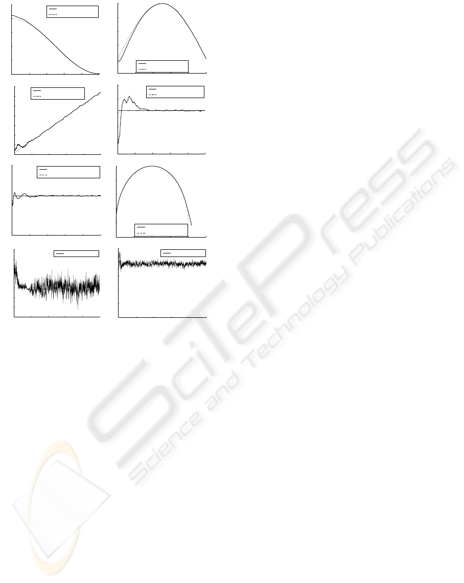
4.1.2 Simulation with uncertainties
Nevertheless, when noise is added, the errors are not
stabilized (Fig. 3). Therefore, control (12) is not ro-
bust with respect to the perturbations. In order to re-
ject noise, the control law is divided into two parts
(11): the ideal control (12) and the discontinuous law
described by (17). Perturbations π
5
and π
6
are noise
of mean 0.1 and of variance 0.1. The matching noise
is bounded and the disturbances k
i
=[K
i,1
,K
i,2
, 0]
T
is the unmatched perturbation which satisfy (19) (i.e.
ρ
i
< 0.2E
i
). In order to avoid the chattering phe-
nomenon, the function signum in (17) is replaced by
2
π
atan (σ
i
) with 1. Using the control law (11)
with D
i
=[0, 0, 1], the tracking errors tend to zero
(Fig. 5) and the system (2) is robust with respect to
perturbation from the initial time (ie. sliding function
σ
i
represented in Fig. 4 is equal to zero from the ini-
tial time).
−40 −20 0 20 4
0
−5
0
5
10
15
20
25
y (m)
x (m)
actual trajectory
desired trajectory
Figure 3: Evolution in the phase plane (x, y) with uncer-
tainties without ISM
0 20 40 60 80 10
0
−0.5
0
0.5
t (s)
σ
1
sliding function
Figure 4: Evolution of the sliding function σ
1
5 CONCLUSION
The problem of robust control design has been con-
sidered for the tracking of a unicycle robot system
with bounded disturbances and uncertainties. The
proposed controller includes terms corresponding to
an integral sliding mode component and enables to
obtain continuous velocity and acceleration inputs for
some practical applications on mechanical systems.
The integral sliding mode component compensates
ICINCO 2005 - ROBOTICS AND AUTOMATION
110
0 20 40 60 80 10
0
−20
−10
0
10
20
30
x (m)
t (s)
actual trajectory
desired trajectory
0 20 40 60 80 10
0
−5
0
5
10
15
20
y (m)
t (s)
actual trajectory
desired trajectory
0 20 40 60 80 10
0
1.5
2
2.5
3
3.5
4
4.5
5
θ (rad)
t (s)
actual orientation
desired orientation
0 20 40 60 80 10
0
0
0.2
0.4
0.6
0.8
1
t (s)
u (m/s)
actual linear speed
desired linear speed
0 20 40 60 80 10
0
−0.5
0
0.5
v
t
actual angular speed
desired angular speed
−20 −10 0 10 20 3
0
−5
0
5
10
15
20
y (m)
x (m)
actual trajectory
desired trajectory
0 20 40 60 80 10
0
−0.4
−0.3
−0.2
−0.1
0
0.1
0.2
0.3
P (m/s
3
)
t (s)
control input P
0 20 40 60 80 10
0
−2
−1.5
−1
−0.5
0
0.5
τ (rad/s
2
)
t (s)
control input τ
Figure 5: Evolution of variables and inputs without noise
using the proposed controller
for the matching perturbation beginning from the ini-
tial time and for some unmatched disturbances. Simu-
lations on a unicycle-type mobile robot illustrated the
performance of the controller.
REFERENCES
Astolfi, A. (1996). Discontinuous control of nonholonomic
systems. Systems and Control Letters, 27:37–45.
Brockett, R. (1983). Asymptotic stability and feedback sta-
bilization. Springer-Verlag.
Cao, W. and Xu, J. (2004). Nonlinear integral type slid-
ing surface for both matched and unmatched uncer-
tain systems. IEEE Trans. on Automatic Control,
49(8):1355–1360.
de Wit, C. C. and Sordalen, O. (1992). Exponential sta-
bilization of mobile robots with nonholonomic con-
straints. IEEE Trans. Automatic Control, 37:1791–
1797.
Edwards, C. and Spurgeon, S. (1998). Sliding mode control:
theory and applications. Taylor and Francis.
Fliess, M., Levine, J., Martin, P., and Rouchon, P. (1995).
Flatness and defect of nonlinear systems : Introduc-
tory theory and examples. Int. Journal of Control,
61:1327–1361.
Floquet, T., Barbot, J.-P., and Perruquetti, W. (2003).
Higher-order sliding mode stabilization for a class
of nonholonomic perturbed systems. Automatica,
39:1077–1083.
Hespanha, J. and Morse, A. (1999). Stabilization of non-
holonomic integrators via logic-based switching. Au-
tomatica, 35:385–393.
Jiang, Z. (2000). Robust exponential regulation of non-
holonomic systems with uncertainties. Automatica,
36:189–209.
Laumond, J. (1998). Robot motion planning and control.
Springer-Verlag.
Monaco, S. and Normand-Cyrot, D. (1992). An introduc-
tion to motion planning under multirate digital con-
trol. In IEEE Conf. on Decision and Control, pages
1780–1785, Tucson, Arizona.
Murray, R. and Sastry, S. (1993). Nonholonomic motion
planning: steering using sinusoids. Transactions on
Automatic Control, 38:700–716.
Perruquetti, W. and Barbot, J.-P. (2002). Sliding mode con-
trol in engineering. Control Eng. Series Vol. 11.
Pomet, J. (1992). Explicit design of time-varying stabilizing
control laws for a class of controllable systems with-
out drift. Systems and Control Letters, 18:147–158.
Poznyak, A., Fridman, L., and Bejarano, F. (2004). Mini-
max integral sliding-mode control for multimodel lin-
ear uncertain systems. IEEE Trans. Automatic Con-
trol, 49:97–102.
Qu, Z. (1998). Robust control of nonlinear uncertain sys-
tems. New York: Wiley.
Samson, C. (1995). Control of chained systems: Ap-
plication to path following and time varying point-
stabilization of mobile robots. IEEE Trans. on Au-
tomatic Control, 40:64–77.
Utkin, V. and Shi, J. (1996). Integral sliding mode in sys-
tems operating under uncertainty conditions. In IEEE
Conf. on Decision and Control, pages 4591–4596,
Kobe, Japan,.
TRACKING OF A UNICYCLE-TYPE MOBILE ROBOT USING INTEGRAL SLIDING MODE CONTROL
111
