CONTRIBUTORS TO A SIGNAL FROM AN ARTIFICIAL

CONTRAST

Jing Hu and George Runger

Arizona State University

Tempe, AZ

Eugene Tuv

Intel Corporation

Chandler, AZ

Keywords:

Patterns, statistical process control, supervised learning, multivariate analysis.

Abstract:

Data from a process or system is often monitored in order to detect unusual events and this task is required in

many disciplines. A decision rule can be learned to detect anomalies from the normal operating environment

when neither the normal operations nor the anomalies to be detected are pre-speciﬁed. This is accomplished

through artiﬁcial data that transforms the problem to one of supervised learning. However, when a large

collection of variables are monitored, not all react to the anomaly detected by the decision rule. It is important

to interrogate a signal to determine the variables that are most relevant to or most contribute to the signal

in order to improve and facilitate the actions to signal. Metrics are presented that can be used determine

contributors to a signal developed through an artiﬁcial contrast that are conceptually simple. The metrics are

shown to be related to traditional tools for normally distributed data and their efﬁcacy is shown on simulated

and actual data.

1 INTRODUCTION

Statistical process control (SPC) is used to detect

changes from standard operating conditions. In multi-

variate SPC a p×1 observation vector x is obtained at

each sample time. Some statistics, such as Hotelling’s

statistic (Hotelling, 1947), have been developed to

detect whether the observation falls in or out of the

control region representing standard operating condi-

tions. This leads to two important comments. First,

the control region is deﬁned through an analytical ex-

pression which is based on the assumption of normal

distribution of the data. Second, after a signal further

analysis is needed to determine the variables that con-

tribute to the signal.

Our research is an extension of the classical meth-

ods in terms of the above two points. The results in

(Hwang et al., 2004) described the design of a control

region based only on training data without a distrib-

utional assumption. An artiﬁcial contrast was devel-

oped to allow the control region to be learned through

supervised learning techniques. This also allowed for

control of the decision errors through appropriate pa-

rameter values. The second question is to identify

variables that are most relevant to or most contribute

to a particular signal. We refer to these variables as

contributors to the signal. These are the variables that

receive priority for corrective action. Many industries

use an out-of-control action plan (OCAP) to react to

a signal from a control chart. This research enhances

and extends OCAP to incorporate learned control re-

gions and large numbers of variables.

A physical event, such as a broken pump or a

clogged pipe, might generate a signal from a con-

trol policy. However, not all variables might react

to this physical event. Instead, when a large collec-

tion of variables are monitored, often only a few con-

tribute tothe signal from the control policy. For exam-

ple, although a large collection of variables might be

monitored, potentially only the pressure drop across a

pump might be sensitive to a clogged pipe. The ob-

jective of this work is to identify these contributors in

order to improve and facilitate corrective actions.

It has been a challenge for even normal-theory

based methods to completely solve this problem. The

key issue is the interrelationships between the vari-

ables. It is not sufﬁcient to simply explore the mar-

ginal distribution of each variable. This is made clear

Hu J., Runger G. and Tuv E. (2005).

CONTRIBUTORS TO A SIGNAL FROM AN ARTIFICIAL CONTRAST.

In Proceedings of the Second International Conference on Informatics in Control, Automation and Robotics, pages 3-10

DOI: 10.5220/0001172900030010

 SciTePress

in our illustrations that follow. Consequently, early

work (Alt, 1985; Doganaksay et al., 1991) required

improvement. Subsequent work under normal theory

considered joint distributions of all subsets of vari-

ables (Mason et al., 1995; Chua and Montgomery,

1992; Murphy, 1987). However, this results in a

combinatorial explosion of possible subsets for even

a moderate number of variables. In (Rencher, 1993)

and (Runger et al., 1996) an approach based on con-

ditional distributions was used that resulted in feasi-

ble computations, again for normally distributed data.

Only one metric was calculated for each variable.

Furthermore, in (Runger et al., 1996) a number of rea-

sonable geometric approaches were deﬁned and these

were shown to result in equivalent metrics. Still, one

metric was computed for each variable. This idea is

summarized brieﬂy in a following section. Although

there are cases where the feasible approaches used in

(Rencher, 1993) and (Runger et al., 1996) are not suf-

ﬁcient, they are effective in many instances, and the

results indicate when further analysis is needed. This

is illustrated in a following section.

The method proposed here is a simple, computa-

tionally feasible approach that can be shown to gen-

eralize the normal-theory methods in (Rencher, 1993)

and (Runger et al., 1996). Consequently, it has the ad-

vantage of equivalence of a traditional solution under

traditional assumptions, yet provides a computation-

ally and conceptually simple extension. In Section 2

a summary is provided of the use of an artiﬁcial con-

trast with supervised learning is to generate a control

region. In Section 3 the metric used for contributions

is presented. The following section present illustra-

tive examples.

2 CONTROL REGION DESIGN

Modern data collection techniques facilitate the col-

lection of in-control data. In practice, the joint distri-

bution of the variables for the in-control data is un-

known and rarely as well-behaved as a multivariate

normal distribution. If speciﬁc deviations from stan-

dard operating conditions are not a priori speciﬁed,

leaning the control region is a type of unsupervised

learning problem. An elegant technique can be used

to transform the unsupervised learning problem to a

supervised one by using an artiﬁcial reference distrib-

ution proposed by (Hwang et al., 2004). This is sum-

marized brieﬂy as follows.

Suppose f(x) is an unknown probability density

function of in-control data, and f

(x) is a speciﬁed

reference density function. Combine the original data

set x

, x

, ..., x

sampled from f

(x) and a random

sample of equal size N drawn from f

(x).If we as-

sign y = −1 to each sample point drawn from f(x)

and y = 1 for those drawn from f

(x), then learning

control region can be considered to deﬁne a solution

to a two-class classiﬁcation problem. Points whose

predicted y are −1 are assigned to the control region,

and classiﬁed into the “standard” or “on-target” class.

Points with predicted y equal to 1 are are classiﬁed

into the“off-target” class.

For a given point x, the expected value of y is

µ(x) = E(y|x) = p(y = 1|x) − p(y = −1|x)

= 2p(y = 1|x) − 1

Then, according to Bayes’ Theorem,

p(y = −1|x) =

p(y = −1|x)

p(x)

p(x| − 1)p(y = −1)

p(x| − 1)p(y = −1) + p(x|1)p(y = 1)

f(x)

f(x) + f

(x)

(1)

where we assume p(y = 1) = p(y = −1) for train-

ing data, which means in estimating E(y|x) we use

the same sample size for each class. Therefore, an

estimate of the unknown density f(x) is obtained as

f(x) =

1 − bµ(x)

1 + bµ(x)

× f

(x), (2)

where f

(x) is the known reference probability den-

sity function of the random data and ˆµ(x)is learned

from the supervised algorithm. Also, the odds are

p(y = −1|x)

p(y = 1|x)

f(x)

(x)

(3)

The assignment is determined by the value of ˆµ(x).

A data x is assigned to the class with density f (x)

when

bµ(x) < v,

and the class with density f

(x) when

bµ(x) > v.

where v is a parameter that can used to adjust the error

rates of the procedure.

Any supervised learner is a potential candidate to

build the model. In our research, a Regularized Least

Square Classiﬁer (RLSC) (Cucker and Smale, 2001)

is employed as the speciﬁc classiﬁer. Squared error

loss is used with a quadratic penalty term on the co-

efﬁcients (from the standardization the intercept is

zero). Radial basis functions are used at each ob-

served point with common standard deviation. That

is the mean of y is estimated from

µ(x) = β

j=1

exp



−

kx − x

/σ



= β

j=1

(x, x

) (4)

ICINCO 2005 - INTELLIGENT CONTROL SYSTEMS AND OPTIMIZATION

Also, let β = (β

, . . . , β

). The β

are estimated

from the penalized least squares criterion

min

,β

i=1

− β

−

j=1

exp

−

kx − x

/σ

+ γkβk

(5)

where n is the total number of observations in the

training data set. If the x’s and y are standardized

to mean zero then it can be shown that

= 0. Also,

let the matrix K denote the n ×n matrix with (i, j)th

element equal to K

, x

). Then for a ﬁxed σ the

solution for β is

β = (K + nγI)

−1

y (6)

and this is used to estimate µ(x).

3 CONTRIBUTORS TO A SIGNAL

In this section, a metric is developed to identify vari-

ables that contribute to a signal from SPC based upon

artiﬁcial contrasts. Suppose there are p correlated

variables (x

, x

, . . . , x

). Let x

∗

be an observed data

point that results in a signal from the control scheme.

Deﬁne the set

= {x|x

= x

∗

, i 6= k}

There are several reasonable metrics for the contri-

bution of variable x

to the out-of-control signal. We

use

∗

) = max

x∈L

f(x)

f(x

∗

)

(7)

This measures the change from

f(x)/

f(x

∗

) that can

be obtained from only a change to x

. If η

∗

) is

small then x

∗

is not unusual. If η

∗

) is large, then a

substantial change can result from a change to x

and

is considered to be an important contributor to the

signal.

From (2) it can be shown that bµ(x) is a monotone

function of the estimated density ratio

f(x)/

(x).

Therefore, the value x

∈ L

that maximizes the es-

timated density ratio also maximizes bµ(x) over this

same set. In the special case that f

(x) is a uniform

density the value of x

∈ L

that maximizes bµ(x)

also maximizes

f(x) over this set. Consequently,

∗

) considers the change in estimated density that

can be obtained from a change to x

From (3) we have that η

is the maximum odds ra-

tio obtained over L

∗

) = max

x∈L

ˆp(y = −1|x)/ˆp(y = 1|x)

ˆp(y = −1|x

∗

)/ˆp (y = 1|x

∗

)

(8)

To compare values of η

∗

) over k the denominator

in (8) can be ignored and the numerator is a monotone

function of ˆp(y = −1|x). Consequently, the value in

that maximizes η

∗

) is the one that maximizes

ˆp(y = −1|x). Therefore, the η

∗

) metric is similar

to one that scores the change in estimated probability

of an in-control point.

A point that is unusual simultaneously in more than

one variable, but not in either variable individually, is

not well identiﬁed by this metric. That is, if x

∗

unusual in the joint distribution of (x

, . . . , x

) for

k ≤ p, but not in the conditional marginal distribu-

tion of f(x

= x

∗

, i 6= j) then the metric is not

sensitive. This implies that the point is unusual in a

marginal distribution of more than one variable. Con-

sequently, one can consider a two-dimensional set

= {x|x

= x

∗

, i 6= j, k}

and a new metric

∗

) = max

x∈L

f(x)

f(x

∗

)

(9)

to investigate such points. This two-dimensional met-

ric would be applied if none of the one-dimensional

metrics η

∗

) are unusual. Similarly, higher-

dimensional metrics can be deﬁned and applied as

needed. The two-dimensional metric η

∗

) would

maximize the the estimated density over x

and x

. It

might use a gradient-based method or others heuris-

tics to conduct the search. The objective is only to

determine the pair of variables that generate large

changes in the estimated density. The exact value

of the maximum density is not needed. This per-

mits large step sizes to be used in the search space.

However, the focus of the work here is to use the

one-dimensional metrics η

∗

)’s. Because the con-

tribution analysis is only applied to a point which

generates a signal, no information for the set of one-

dimensional η

’s implies that a two-dimensional (or

higher) metric needs to be explored. However, the

one-dimensional η

’s are effective in many cases, and

they provide a starting point for all cases.

3.1 Comparison with a Multivariate

Normal Distribution

In this section, we assume the variables follow a mul-

tidimensional normal distribution. Under these as-

sumptions, we can determine the theoretical form of

the metric η

∗

). Given the estimate of the unknown

density

f(x), deﬁne x

= argmax

x∈L

f(x)

For a multivariate normal density with mean vector µ

and covariance matrix Σ

= argmin

x∈L

(x − µ)

′

−1

(x − µ)

Therefore, x

is the point in L

at which Hotelling’s

statistic is minimized. Consequently, x

is the same

CONTRIBUTORS TO A SIGNAL FROM AN ARTIFICIAL CONTRAST

point used in (Runger et al., 1996) to deﬁne the contri-

bution of variable x

in the multivariate normal case.

The use of the metric in (7) generalizes this previous

result from a normal distribution to an arbitrary distri-

bution.

4 ILLUSTRATIVE EXAMPLE

4.1 Learning the In-Control

Boundary

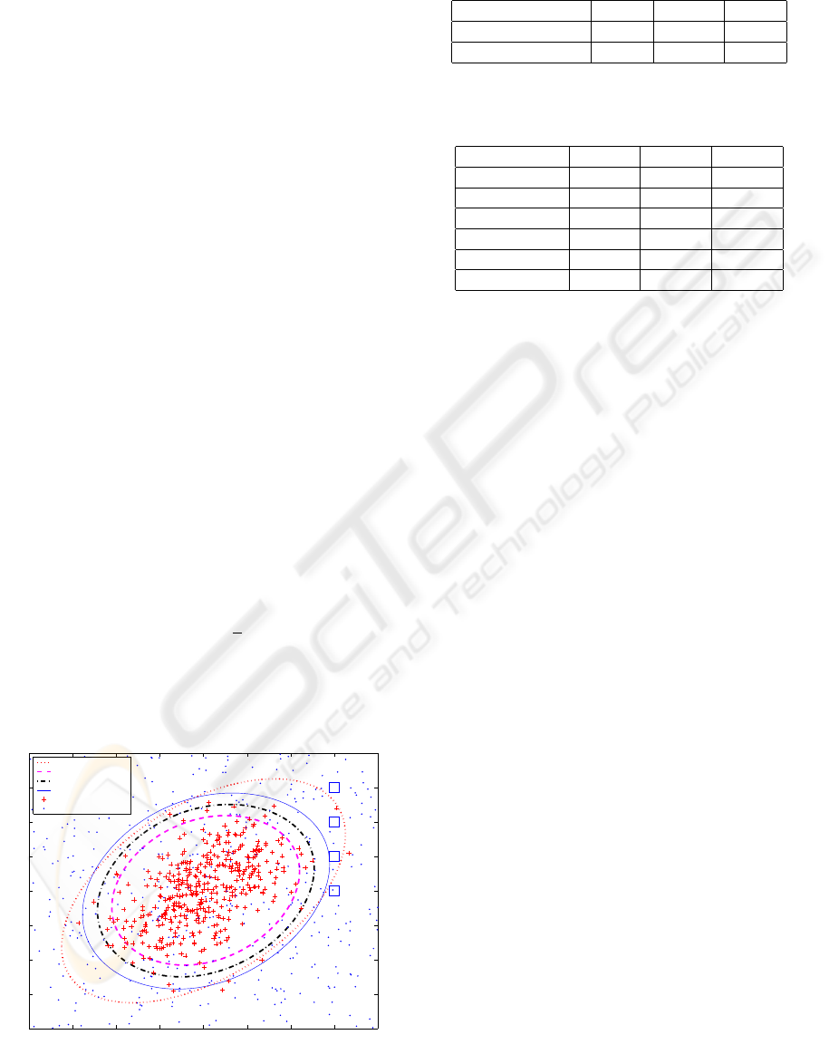
To demonstrate that our method is an extension of the

traditional method, ﬁrst we assume that the in-control

data follow a multivariate normal distribution. In the

case of two variables, we capture a smooth, closed

elliptical boundary. Figure (1) shows the boundary

learned through an artiﬁcial contrast and a supervised

learning method along with the boundary speciﬁed

by Hotelling’s statistic (Hotelling, 1947) for the in-

control data.

The size of in-control training data is 400 and the

size of uniform data is also 400. The in-control train-

ing data are generated from the two-dimensional nor-

mal distribution X = C ∗ Z with covariance

Cov(X) = CC

′



1 0.5

0.5 1



and Z following two-dimensional joint standardized

normal distribution with ρ = 0. The smoothing para-

meter for the classiﬁer is γ = 4/800. The parameter

for the kernel function is σ =

√

8. The out-of-control

training data are generated from the reference distri-

bution. There are four unusual points: A (3, 0), B

(3, 1), C (3, 2), and D (3, 3).

−4 −3 −2 −1 0 1 2 3 4

−4

−3

−2

−1

Boundaries

Tsquare: α=0.005

Constrast: cutoff=0

Constrast: cutoff=0.2

Constrast: cutoff=0.4

in−control data

out−of−control data

Figure 1: Learned Boundaries and Hotelling’s Boundary

Table 1: Type I error for In-control Data

cut-off value 0 0.2 0.4

the training data 0.085 0.0325 0.015

the testing data 0.1 0.0525 0.025

Table 2: Type II error for Out-of-control Data with Different

Shifted Means

cut-off value 0 0.2 0.4

(1,0) 0.785 0.895 0.96

(1,1) 0.7275 0.8325 0.8975

(2,0) 0.4875 0.6125 0.7325

(2,2) 0.3225 0.45 0.565

(3,0) 0.1025 0.215 0.325

(3,3) 0.055 0.1025 0.185

Testing data sets are used to evaluate performance,

that is, Type I error and Type II error of the classiﬁer.

They are generated from similar multivariate normal

distributions with or without shifted means. Each test-

ing data set has a sample size of 400.

Table 1 gives the Type I error for the training data

and for the testing data whose mean is not shifted. It

shows that the Type I error decreases when the cut-

off value of the boundary increases. Table 2 gives the

Type II error for the testing data with shifted mean. It

shows that for a given shift, the Type II error increases

when the cut-off value of the boundary increases. It

also illustrates that, for a given cut-off value, the fur-

ther the mean shifts from the in-control mean, the

lower the Type II error.

4.2 Contribution Evaluation

The probability density function of the in-control data

f(x) is estimated by (2). For the normal distribution

in Section 3.1 examples are provided in the cases of

two-dimensions (Figure 2)and 30-dimensions (Figure

3).

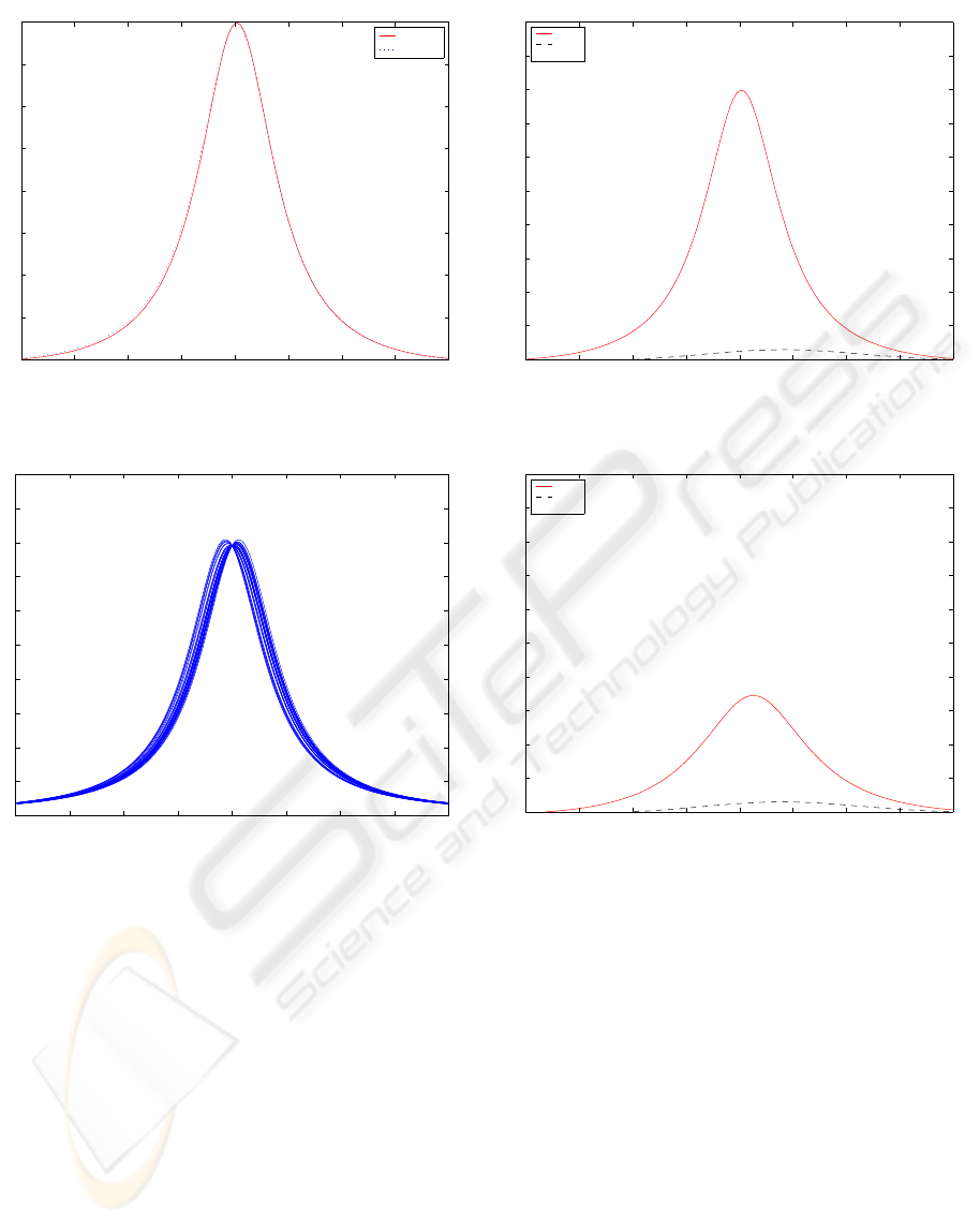
For the case of two dimensions, Figure (1) shows 4

points at (3, 0), (3, 1), (3, 2), (3, 3). The correspond-

ing curves for

f(x) for each point are shown in Fig-

ure (4) through Figure (7). These ﬁgures show that

the variable that would be considered to contribute

to the signal for points (3, 0) and (3, 1) is identiﬁed

by the corresponding curve. For point (3, 2) the vari-

able is not as clear and the curves are also ambiguous.

For the point (3, 3) both variables can be considered

to the signal and this is indicated by the special case

where all curve are similar. That is, no proper subset

of variables is identiﬁed and this is an example where

a higher-dimensional analysis (such as with η

∗

))

is useful.

ICINCO 2005 - INTELLIGENT CONTROL SYSTEMS AND OPTIMIZATION

−4 −3 −2 −1 0 1 2 3 4

0.02

0.04

0.06

0.08

0.1

0.12

0.14

0.16

Based on Means

f(x

,mu

)

f(mu

)

Figure 2: Density estimate for two dimensions

−4 −3 −2 −1 0 1 2 3 4

0.5

1.5

2.5

3.5

4.5

x 10

−26

Based on Means

Figure 3: Density estimate for thirty dimensions

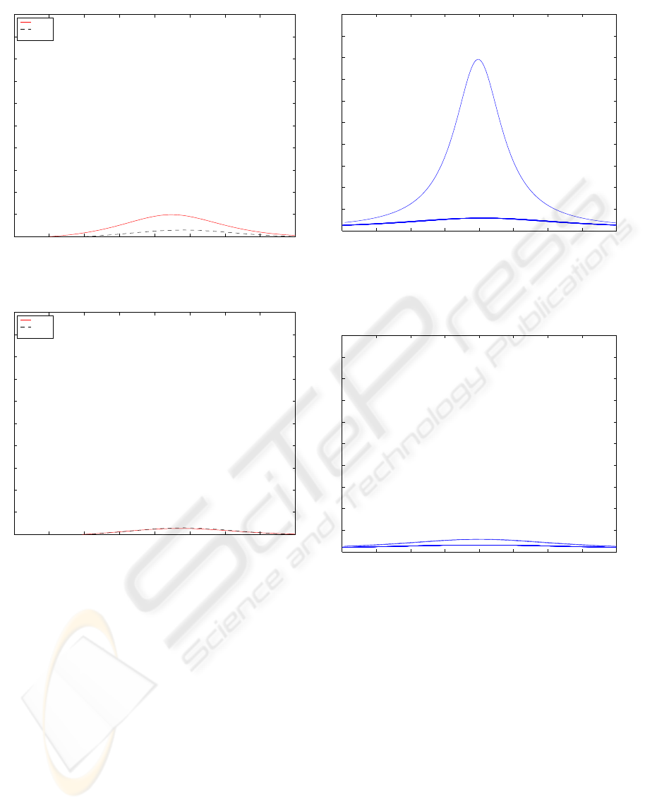
4.3 Example in 30 Dimensions

For a higher dimensional example, consider p = 30

dimensions. Out-of-control points are generated and

density curves are produced for each variable. These

curves are proportional to the conditional density with

all the other variables at the observed values. For p =

30 the size of in-control training data is 200 and the

size of the uniform data is also 200. Curves for out-

of-control points

A = (3, 0, . . . , 0)

B = (3, −3, 0, . . . , 0)

C = (3, 3, . . . , 3)

are generated. For p = 30 dimensions the density

curves are shown in Figure (8) through Figure (10).

−4 −3 −2 −1 0 1 2 3 4

0.02

0.04

0.06

0.08

0.1

0.12

0.14

0.16

0.18

0.2

Based on Values

k=1

k=2

(3 0)

Figure 4: f(x

, 0) and f (3, x

)

−4 −3 −2 −1 0 1 2 3 4

0.02

0.04

0.06

0.08

0.1

0.12

0.14

0.16

0.18

0.2

Based on Values

k=1

k=2

(3 1)

Figure 5: f(x

, 1) and f (3, x

)

Note that the changes in density match the contrib-

utors to an unusual point. Note that for point C the

density metric does not indicate any subset of vari-

ables as contributors. This is a special case and such a

graph implies that all variables contribute to the signal

from the chart because these graphs are only gener-

ated after a signal from a control has been generated.

Such a special case is also distinguished from cases

where only a proper subset of variables contribute to

the signal.

For the particular case of p = 30 dimensions,

values of η

) are calculated for these points and

k = 1, . . . , 30 in Figure (11) through Figure (13).

The results indicate the this metric can identify vari-

ables that contribute to the signal. For point C simi-

lar comments made for the density curves apply here.

The metric does not indicate any subset of variables as

contributors. This is a special case and such a graph

CONTRIBUTORS TO A SIGNAL FROM AN ARTIFICIAL CONTRAST

−4 −3 −2 −1 0 1 2 3 4

0.02

0.04

0.06

0.08

0.1

0.12

0.14

0.16

0.18

0.2

Based on Values

k=1

k=2

(3 2)

Figure 6: f(x

, 2) and f (3, x

)

−4 −3 −2 −1 0 1 2 3 4

0.02

0.04

0.06

0.08

0.1

0.12

0.14

0.16

0.18

0.2

Based on Values

k=1

k=2

(3 3)

Figure 7: f(x

, 3) and f (3, x

)

implies that all variables contribute to the signal from

the chart.

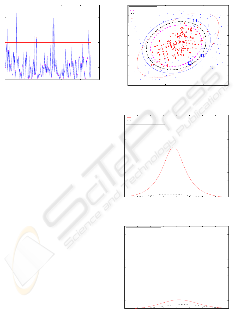
5 MANUFACTURING EXAMPLE

The data set was from a real industrial process. There

are 228 samples in total. To illustrate our problem,

we use two variables. Here, Hotelling T

is employed

to ﬁnd out in-control data. The mean vector and co-

variance matrix are estimated from the whole data set

and T

follows a χ

distribution with two degrees of

freedom. The false alarm, α, is set as 0.05 in order

to screen out unusual data. Figure (14) displays the

Hotelling T

for each observation. From the results,

we obtain 219 in-control data points that are used as

the training data.

−4 −3 −2 −1 0 1 2 3 4

0.5

1.5

2.5

3.5

4.5

x 10

−26

Based on ValuesPoint 1

k=1

Figure 8: Density f(x) as a function of x

for k =

1, 2, . . . , 30 for Point A

−4 −3 −2 −1 0 1 2 3 4

0.5

1.5

2.5

3.5

4.5

x 10

−26

Based on ValuesPoint 2

k=1

k=2

Figure 9: Density f(x) as a function of x

for k =

1, 2, . . . , 30 for Point B

Figure (15) shows the learned boundaries with dif-

ferent cut-off values and the Hotelling T

boundary

with α being 0.005. The learned boundary well cap-

tures the characteristic of the distribution of the in-

control data. We select the learned boundary with

cut-off v = 0.4 as the decision boundary and obtain

three unusual points: Point 1, 2, and 4. The metric is

applied to Point 2 and 4 and Table (3) and it demon-

strates η values for each dimension for each point.

Figure (16) and Figure (17) demonstrate f(x

, x

)

when as functions of x

and x

for Point 2 and 4,

respectively. For Point 2, η

is signiﬁcantly larger

than η

so the ﬁrst variable contributes to the out-of-

control signal. For Point 4, η

and η

are close so both

variables contributes to the out-of-control signal.

ICINCO 2005 - INTELLIGENT CONTROL SYSTEMS AND OPTIMIZATION

−4 −3 −2 −1 0 1 2 3 4

0.5

1.5

2.5

3.5

4.5

x 10

−26

Based on ValuesPoint 3

Figure 10: Density f (x) as a function of x

for k =

1, 2, . . . , 30 for Point C

0 5 10 15 20 25 30

Dimension

Based on Values: Point 3

Figure 11: Contributor metric η

for variables k =

1, 2, . . . , 30 for Point A

6 CONCLUSION

A supervised method to learn normal operating con-

ditions provides a general solution to monitor systems

of many types in many disciplines. In addition to

the decision rule it is important to be able to inter-

rogate a signal to determine the variables that con-

tribute to it. This facilitates an actionable response

to a signal from decision rule used to monitor the

process. In this paper, contributors to a multivari-

ate SPC signal are identiﬁed from the same func-

tion that is learned to deﬁne the decision rule. The

approach is computationally and conceptually sim-

ple. It was shown that the method generalizes a tra-

ditional approach for traditional multivariate normal

theory. Examples show that the method effectively re-

0 5 10 15 20 25 30

Dimension

Based on Values: Point 3

Figure 12: Contributor metric η

for variables k =

1, 2, . . . , 30 for Point B

0 5 10 15 20 25 30

Dimension

Based on Values: Point 3

Figure 13: Contributor metric η

for variables k =

1, 2, . . . , 30 for Point C

produces solutions for known cases, yet it generalizes

to a broader class of problems. The one-dimensional

metric used here would always be a starting point for

such a contribution analysis. Future work is planned

to extend the metric to two- and higher-dimensions

to better diagnose contributors for cases in which the

one-dimensional solution is not adequate.

Table 3: η for Point 2 and 4

Point 2 16.791 1.0001

Point 4 3.6737 1.6549

CONTRIBUTORS TO A SIGNAL FROM AN ARTIFICIAL CONTRAST

0 50 100 150 200 250

Hotelling Tsquare Chart, UCL=5.9915

Figure 14: Hotelling T

REFERENCES

Alt, F. B. (1985). Multivariate quality control. In Kotz, S.,

Johnson, N. L., and Read, C. R., editors, Encyclope-

dia of Statistical Sciences, pages 110–122. John Wiley

and Sons, New York.

Chua, M. and Montgomery, D. C. (1992). Investigation and

characterization of a control scheme for multivariate

quality control. Quality and Reliability Engineering

International, 8:37–44.

Cucker, F. and Smale, S. (2001). On the mathematical foun-

dations of learning. Bulletin of AMS, 39:1–49.

Doganaksay, N., Faltin, F. W., and Tucker, W. T. (1991).

Identiﬁcation of out-of-control quality characteris-

tics in a multivariate manufacturing environment.

Communications in Statistics-Theory and Methods,

20:2775–2790.

Hotelling, H. (1947). Multivariate quality control-

illustrated by the air testing of sample bombsights.

In Eisenhart, C., Hastay, M., and Wallis, W., edi-

tors, Techniques of Statistical Analysis, pages 111–

184. McGraw-Hill, New York.

Hwang, W., Runger, G., and Tuv, E. (2004). Multivariate

statistical process control with artiﬁcial contrasts. un-

der review.

Mason, R. L., Tracy, N. D., and Young, J. C. (1995). De-

composition of T

for multivariate control chart inter-

pretation. Journal of Quality Technology, 27:99–108.

Murphy, B. J. (1987). Selecting out-of-control variables

with T

multivariate quality control procedures. The

Statistician, 36:571–583.

Rencher (1993). The contribution of individual variables to

hotelling’s T

, wilks’ Λ, and R

. Biometrics, 49:479–

489.

Runger, G. C., Alt, F. B., and Montgomery, D. C. (1996).

Contributors to a multivariate control chart signal.

Communications in Statistics - Theory and Methods,

25:2203–2213.

−4 −3 −2 −1 0 1 2 3 4

−4

−3

−2

−1

Boundaries

Tsquare: α=0.005

Constrast: cutoff=0

Constrast: cutoff=0.2

Constrast: cutoff=0.4

in−control data

out−of−control data

Figure 15: Learned Boundaries and Hotelling T

−4 −3 −2 −1 0 1 2 3 4

0.02

0.04

0.06

0.08

0.1

0.12

0.14

0.16

0.18

0.2

Based on Values

k=1

k=2

Point 2 : (−2.9758 −0.51562)

Figure 16: Density f(x) as a function of x

and x

for Point

−4 −3 −2 −1 0 1 2 3 4

0.02

0.04

0.06

0.08

0.1

0.12

0.14

0.16

0.18

0.2

Based on Values

k=1

k=2

Point 4 : (2.492 1.9968)

Figure 17: Density f(x) as a function of x

and x

for Point

ICINCO 2005 - INTELLIGENT CONTROL SYSTEMS AND OPTIMIZATION