AN EXPLORATION MEASURE OF THE DIVERSITY

VARIATION IN GENETIC ALGORITHMS

G. A. Papakostas, Y. S. Boutalis

Democritus University of Thrace, Department of Electrical and Computer Engineering, 67100 Xanthi, Hellas

D. A. Karras

Chalkis Institute of Technology, Automation Dept. and Hellenic Open University, Ano Iliupolis, Athens 16342, Hellas

B. G. Mertzios

Thessaloniki Institute of Technolog, Department of Automation, Laboratory of Control Sys. and Comp. Intell., Hellas

Keywords: Genetic Algorithms, Diversity, Clustering.

Abstract: In this paper, a novel measure of the population diversity of a Genetic Algorithm (GA) is presented.

Chromosomes diversity plays a major role for the successfully operation of a GA, since it describes the

number of the different candidate solutions that the algorithm evaluates, in order to find the optimal one, in

respect to a performance index, called objective function. In a well defined algorithm, the diversity of the

current population should be measurable, in order to estimate the performance of the algorithm. The resulted

observation, that is, the measuring of the diversity, can then be used to real-time adjust the factors that

determine the chromosomes variety (P

, P

), during the execution of the GA. It is shown, that a simple

chromosomes clustering into the search space, by using the well known k-means algorithm, can give a

useful picture of the population’s distribution. Thus, by translating the problem of finding the best solution

to a GA-based problem into an iterative clustering process, and by using the scatter matrices (S

, S

), which

describe completely the candidate’s solutions topology, one could define a novel formula that gives the

population diversity of the algorithm.

1 INTRODUCTION

Evolutionary Algorithms (EAs) have been used in

many applications through the years, due to its

stochastic mechanism for finding solutions that

optimize single or multiple objective problems.

Genetic Algorithms (Holland, 2001, Mitchell, 2002)

are considered the most popular kind of EAs since

they are characterized by a high degree of parallism

and natural behaviour.

Genetic Algorithms (GAs) are used as

optimization methods to solve difficult and complex

problems in a range of scientific fields, such as

image processing (Mirmehdi, 1997, Papakostas,

2003), robust control (Jamshidi, 2003, Papakostas,

2004), pattern

classification (Bandyopadhyay, 1995)

etc. Their popularity can be justified by their ability

to overcome possible local optima, and to converge

to the global solution of a problem, with high

probability.

However, there are some cases in which the

global optimum is quite far from the derived

solution that the algorithm converged to. This

undesirable situation is called premature

convergence (Mitchell, 2002). When this

phenomenon appears, the population chromosomes

are all the same. In other words, the population

diversity has been lost. Of course, the diversity

would be also lost in the case of the algorithm

converging to the global optimum. The ill-posed

situation is when the diversity

decreases quickly and

stays to low level for many generations.

Therefore, in order to prevent this situation, it is

needed to measure the diversity variation through

the generations, and adjust the algorithm parameters

off-line, in the initial calibration or online during the

execution of the algorithm.

260

A. Papakostas G., S. Boutalis Y., A. Karras D. and G. Mertzios B. (2005).

AN EXPLORATION MEASURE OF THE DIVERSITY.

In Proceedings of the Second International Conference on Informatics in Control, Automation and Robotics, pages 260-265

 SciTePress

In the present paper, a clustering method for

exploring the distribution of the chromosomes and

the scatter matrices, S

– between class scatter

matrix and S

– within class scatter matrix of the

resulted clusters for measuring the level of the

current diversity, are being used.

The paper is organized as follows: the proposed

method is described in section 2, by analyzing the k-

means algorithm and the way it is used for this paper

purpose, while the effectiveness of the method is

examined through appropriate simulations in the

third section. Finally, conclusions that may derive

from the previous discussion are highlighted in the

last section.

2 THE PROPOSED METHOD

The main idea of the proposed method, for

measuring the population diversity of a GA, is based

on viewing the process to find the optimal solution

of a problem, as a clustering one. Let us consider the

algorithm’s chromosomes for an n-dimensional

problem

)...(...,),...(

321

mmm

xxxxChxxxxCh

where Ch

is the i

chromosome, and

x is the j

variable of the i

chromosome. In the above

formulation, the population size is equal to m.

These chromosomes can be considered as n-

dimensional vectors with coordinates (x

,…,x

and thus can be considered as single points into the

n-dimensional variable space (search space). To

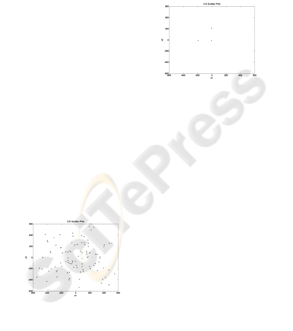
visualize these points in the search space, one can

produce the scatter plot of them, as depicted in the

following figure, where the points correspond to the

initial population in the case of a 2-D problem.

Figure 1: 2-D scatter plot of the initial algorithm’s

population

Assuming that the above figure represents the

location of the initial population of the algorithm,

during the operation of the GA all the chromosomes

tend to converge to the same point of the search

space. As the algorithm converges to an optimum

(global or local), the form of the scatter plot will be

similar to the one of Figure 2.

Figure 2: 2-D scatter plot of the final algorithm’s

population

As can be seen in Figure 2, the diversity of the

final population has significantly decreased over the

generations, since there are only three different

chromosomes. If the solution given by the algorithm

is the global optimum, then the diversity reduction is

acceptable. However, in most of the cases where the

problem to be solved is quite complex, the global

optimum is unknown. It is therefore desirable to

keep the diversity in high levels during the

optimization procedure, in order to explore the

search space as much as possible. Such a strategy

can guarantee the suitability of the current solution,

by high probability.

In the current work, a clustering method is

applied, in order to investigate the location of the

entire population inside the variable space, and the

diversity of the population is measured by means of

the scatter matrices of the resulted chromosome

clusters.

In the next section a brief description of the k-

means clustering algorithm, is taking place, while

the proposed diversity measure is defined, later.

2.1 k-means Algorithm

Clustering methods have many applications in the

engineering science, where data analysis is involved.

In the following, a short definition, of what

clustering stands for, is presented.

Definition 1. Clustering of a given data set, in N-

dimensional space, is the process that partitions

these data into a number of groups (clusters) by

means of a similarity or dissimilarity metric

(Fukunaga, 1990).

AN EXPLORATION MEASURE OF THE DIVERSITY VARIATION IN GENETIC ALGORITHMS

261

One of the most used clustering algorithms is the

k-means one (Looney, 1997), which can be

described in the following steps:

Step 1: Choose K initial cluster centers, C

, C

… C

Step 2: Classify each point of the data set to a cluster

according to the following statement: point x

belongs to cluster i

with center C

, if

jiKji

tCxtCx

≠=∀

−≤−

,,...,2,1,

,)()(

Step 3: Compute the new cluster centers according

Kix

,...,2,1,

)1( ==+

∑

∈

where N

is the number of points belong to the i

cluster

Step 4: If C

(t+1)=C

(t), for i=1,2,..,K, then

algorithm is terminated, otherwise goes to step 2.

It must be noted, that the initialization of the

cluster centers, play major role to the performance

and the fast convergent of the algorithm.

In the proposed method, the k-means algorithm

is applied in each generation to cluster the

population chromosomes. In our approach, two

essential assumptions about this algorithm have been

made:

Assumption 1: The initial number K of the cluster

centers are chosen to be equal to the population

size.

Assumption 2: In each iteration of the k-means

algorithm, the empty clusters are being discarded.

Assumption 1 is being justified by Remark 1 of

the next section, while assumption 2 is made to

prevent the increasing of the clusters number, by

keeping the empty ones, which stay empty until the

end of the algorithm.

2.2 Diversity Measure

Once the clustering is applied on each generation of

the GA, a number of clusters are obtained. The

number and the relative location of these clusters

can be used to measure the diversity of the

algorithm.

A high diversity is presented by a population

which covers the search space as much as possible,

while the low diversity is presented by a population

with all chromosomes being the same. These main

concepts can be declared by Remark 1 and 2

respectively, in terms of clustering.

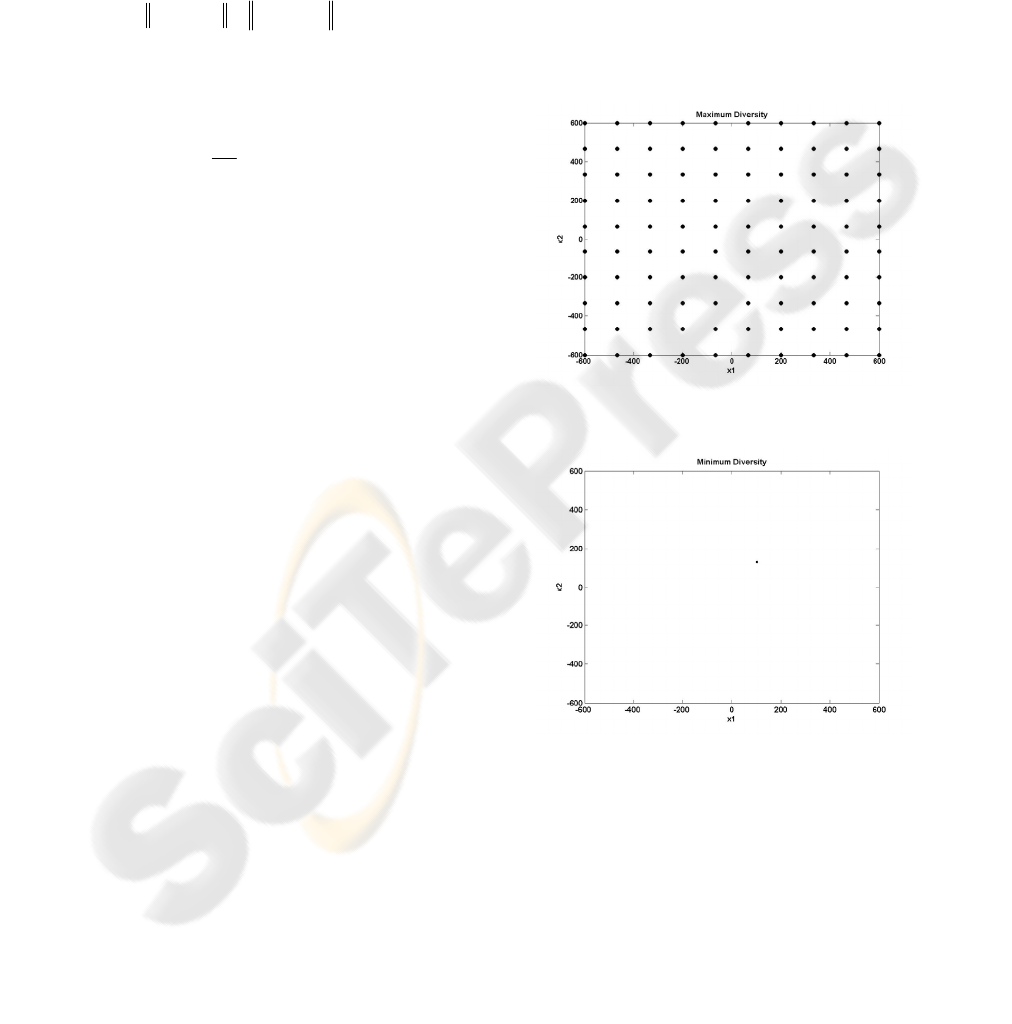
Remark 1: The highest diversity appears when each

chromosome constitutes the center of a cluster with

one member, the chromosome itself and they are

equally spaced, with maximum permit able distance

over the search space (Figure 3).

Remark 2: The lowest diversity appears when all

the chromosomes of the population are the same.

This means that there is one cluster with all the

chromosomes being the center (Figure 4).

Figure 3: 2-D Maximum Diversity, by optimal

chromosomes arrangement

Figure 4: 2-D Minimum Diversity

The above figures correspond to the extreme

situations a GA can be found. In practice, the

algorithm, never presents the diversity illustrated in

Figure 3, but it begins with a random chromosomes

arrangement (Figure 1) and it decreases its diversity

generation by generation. When, the algorithm

terminates, its diversity looks like this of Figure 2, or

this of Figure 4 for full convergence.

To measure these variations of the chromosomes

diversity, the scatter matrices S

and S

(Fukunaga,

1990), are used, when the clustering has finished.

ICINCO 2005 - INTELLIGENT CONTROL SYSTEMS AND OPTIMIZATION

262

Between clusters scatter matrix S

, describes

how the data clusters, obtained by clustering, are

distributed along the search space, and can be

calculated by using the following equation

()()

∑

−−=

iib

mmmmS

where K is the number of clusters obtained from k-

means algorithm, m

is the mean value of the

chromosomes belong to cluster i, and m the mean

value of the entire population.

Within clusters scatter matrix, S

, measures the

distribution of the chromosomes inside the clusters

that they belong, and is described by the equation

()()

ijw

mChmChS

−−=

∑∑

−=11

where N

is the number of chromosomes belonging

to the cluster i and Ch

the j

chromosome. The

remaining symbols are the same as in S

In the previous equations the quantities are

vectors in

ℜ

, according to the problem’s

dimensionality.

Keeping in mind the above definitions of the

scatter matrices, Remark 1 and 2, can be restated as

Remark 3 and 4, below

Remark 3: High diversity occurs when the between

clusters scatter matrix S

, takes its optimal value for

a number of clusters equal to the population size,

and simultaneously the within clusters scatter matrix

, is zero.

Remark 4: Low diversity occurs when the between

clusters scatter matrix S

, is zero meaning that the

number of clusters is equal to one, and

simultaneously the within clusters scatter matrix S

is zero.

Remark 5 is a direct consequent of the above

remarks:

Remark 5: All the intermediate cases are

characterized by random values of S

, S

and

number of clusters.

In order to represent the situations described by

Remark 1 and 2, by a measurable quantity, the

following measure diversity is introduced.

()

(

)

()()

1log1log +++=

StrStrDiversity

where N

is the number of clusters obtained by the

clustering algorithm and tr() the trace of the matrix .

This measure takes high values as N

and tr(S

)

increases, while tr(S

) decreases, thus the Remark 3

is satisfied.

The minimum value of this measure appears in

the case presented in Figure 4, and is equal to zero,

since S

=0, and S

=0.

The above measure has been applied to explore

the diversity of the population, which is being used

to optimize a benchmark function, over the

generations.

The simulations being presented in the next

section, establish the novel diversity measure, a

significant measure to investigate and visualize the

variety of the algorithm population.

3 SIMULATION RESULTS

The experimental results presented here, justify the

usefulness of the proposed diversity measure, in

supervising the progress of a GA.

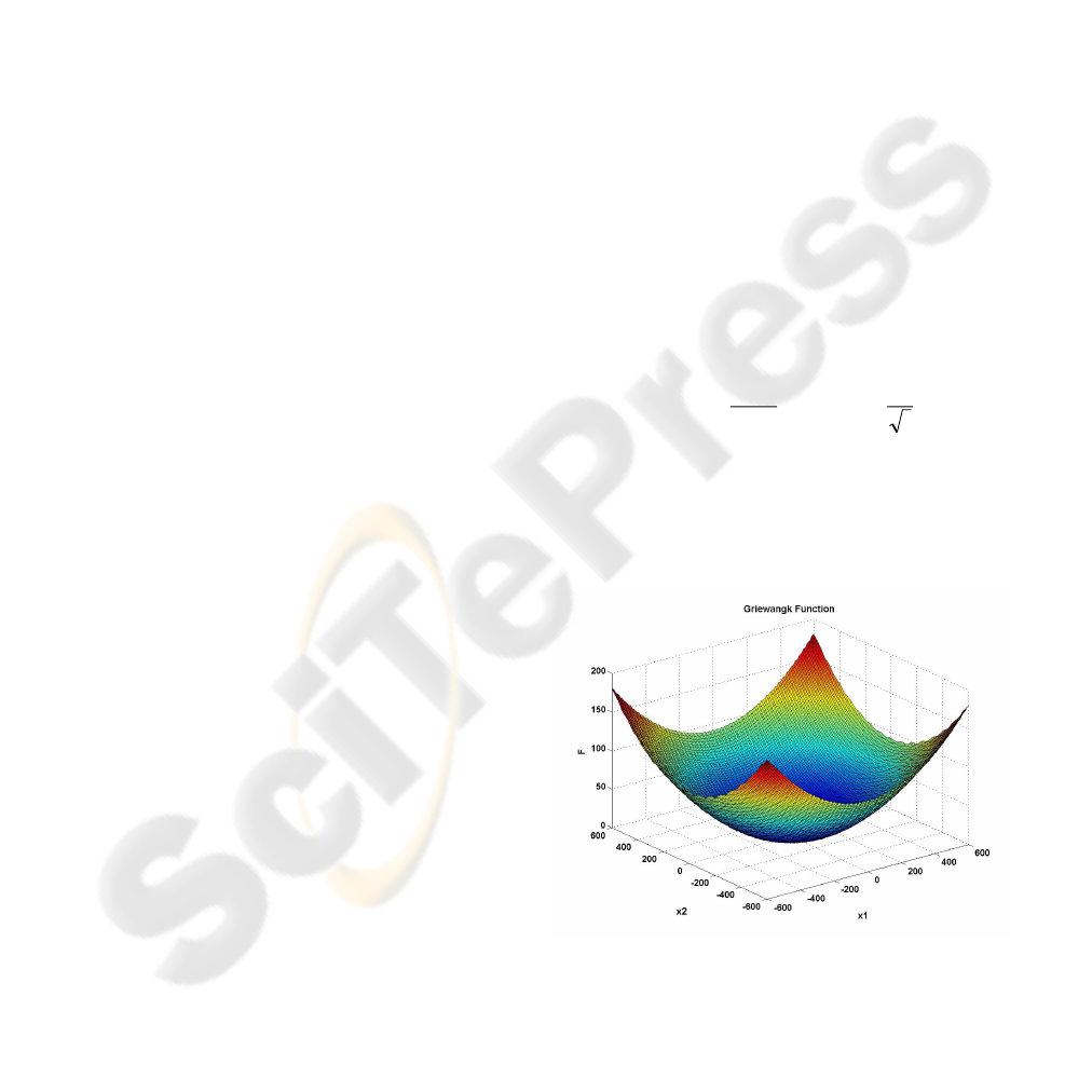
The previous figures are generated by the

optimization of a known benchmark function, the

Griewangk’s function (Digalakis2000). This

function has the following form for two variables

600600

cos

4000

≤≤−

⎟

⎠

⎞

⎜

⎝

⎛

⎟

⎠

⎞

⎜

⎝

⎛

−

⎟

⎠

⎞

⎜

⎝

⎛

∏

∑

Griewangk’s function is multimodal, but the

location of the minima are regularly distributed, as

illustrated in Figure 5,

Figure 5: Griewangk’s function for 2 dimensions

The algorithm used for these experiments is

configured according to the following Table 1.

AN EXPLORATION MEASURE OF THE DIVERSITY VARIATION IN GENETIC ALGORITHMS

263

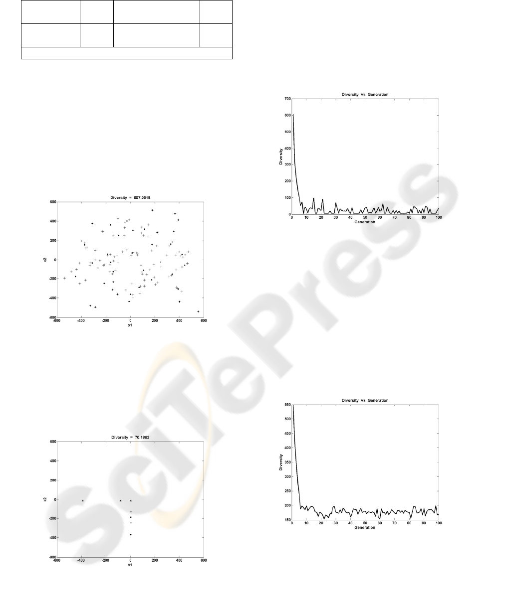
Table 1: GA Parameters

Population

Size

100 Crossover

Probability (P

)

0.8

Selection

Method

SUS Mutation

Probability (P

)

0.01

Generations 100

The simulations are based on the observations of

the minimization process of the above function,

using a simple real-valued GA. During the

execution, the population diversity in each

generation is measured by using, the previously

introduced formula.

Let us investigate the progress of the GA, in

optimizing the Griewangk’s function. The algorithm

starts with a random population and diversity

measure, as depicted in Figure 6.

Figure 6: Initial population with Diversity = 607.0518

As the above figure shows, the cluster centers

(dots) and the chromosomes (plus signs) cover a

large area of the search space, and thus they provide

high diversity measure.

In Figure 7, the scatter plot of the 30

generation’s population is presented.

Figure 7: 30

generation’s population Diversity = 70.1862

It is obvious from the above Figures 6-7, that the

diversity of the population has been lost, after 30

generations. If the minimum has been reached, the

goal has been achieved. In the specific case, the

minimum after 30 generations is 0.5115, quite far

from the global minimum, which is 0.

Thus, the measured diversity can be useful in

changing the crossover and mutation probabilities, in

order to converge to the global minimum.

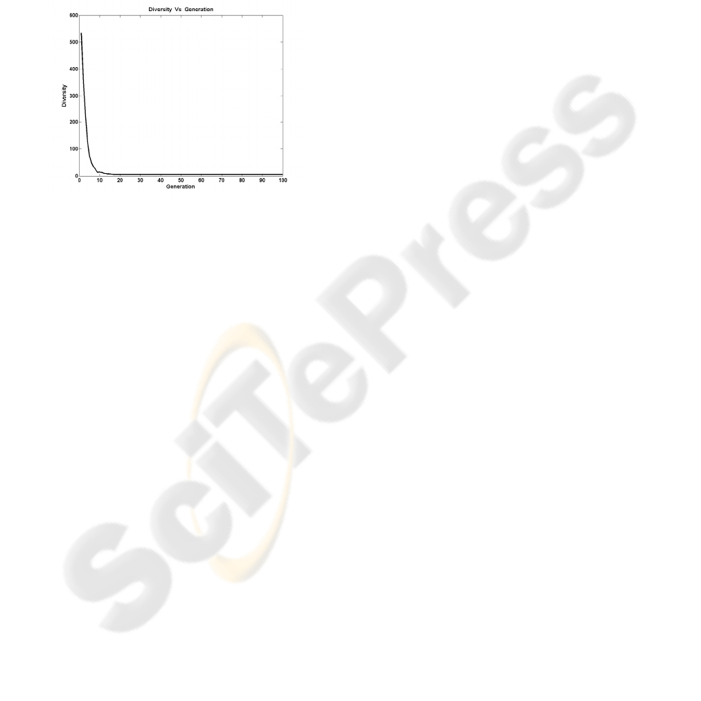
Figure 8, shows the variation of the diversity

through the generations

Figure 8: Diversity variation of the algorithm (Pm=0.01)

For the rest of the generations, the diversity is

varied in low levels, decreasing the probability to

find the global optimum. If the diversity stays in

high levels this probability is increased.

Therefore, the diversity measure proposed in this

paper seems to have the ability to describe the

evolution of the algorithm’s population.

It is very interesting to investigate, the behaviour

of the algorithm in terms of the diversity, by

changing the crossover and mutation probabilities P

and P

, respectively.

Figure 9, presents the diversity variation, for

=0.1.

Figure 9: Diversity variation of the algorithm (P

=0.1)

Mutation probability (P

) controls the

appearance of the search space points that might

have not been presented before. In other words, it

manages to generate all the possible search space

points, by some probability. Thus, it tries to keep the

ICINCO 2005 - INTELLIGENT CONTROL SYSTEMS AND OPTIMIZATION

264

diversity in high levels, a fact that is proved by the

form of the diversity variation of Figure 9. As, can

be seen from this figure, the diversity fluctuates

between 100 and 200, while in the case of P

=0.01,

it varies between 5 and 50.

On the other hand, crossover probability (P

defines the probability by which the chromosomes

interchange their information, in order to produce

better individuals. This probability is changed to 0.5,

in the initial algorithm and the measured diversity is

drawing in Figure 10

Figure 10: Diversity variation of the algorithm (P

=0.5)

Crossover probability determines the population

diversity, by a high degree, as displayed in Figure

10, since a reduction of the crossover probability has

led to premature convergence.

It must be noted that, each one of these

experiments is executed for 100 times, and the mean

diversity has been presented in the above figures.

Additionally, Figures 9 and 10 have been obtained

by applying only one of the operators (crossover,

mutation) each time, during the algorithm execution.

These simulations demonstrates, that the

behaviour of the GA and the impact the crossover

and mutation probabilities have, can be represented

by the diversity measure introduced in this paper.

4 CONCLUSIONS

An innovative formula, which measures the diversity

of GA’s population, has been introduced in the

previous sections. The diversity measure is based on

the statistical quantities that describe the

chromosome clusters obtained by applying the k-

means algorithm to the chromosomes population

The resulted measurement can be used to

calibrate the GA by choosing the appropriate

crossover P

and mutation P

probabilities.

Additionally this measurement will be useful in

adjusting the probabilities on-line during the

execution of the algorithm, in order to keep the

diversity in high levels.

Appropriate experiments have shown that the

proposed measure describes the evolution of the

algorithm’s population. This measure can also be

used to any population-based algorithm, since it uses

the statistical properties of the population’s

distribution over the search space.

Future work must be carried out in order to use

this measure to adaptively adjust the crossover and

mutation probabilities. Additional experiments with

more complex optimization problems such as Neural

Networks training by using GAs must be done. The

training phase of a Neural Network is a process that

is quite blind, because the only measure that one

may have is the approximation error, and due to the

high dimensionality the investigation of the weights

evolution is not possible.

REFERENCES

Bandyopadhyay, S., Murthy, C.A., Pal, S.K., 1995,

Pattern Classification with Genetic Algorithms,

Pattern Recognition Letters, (16), pp. 801-808.

Digalakis, J.G., Margaritis, K.G., 2000, On Benchmarking

Functions for Genetic Algorithms, Int. Journal

Computer Math., Vol.00, pp. 1-27.

Fukunaga, K., 1990, Introduction to Statistical Pattern

Recognition, 2

edition, Academic Press.

Holland, J.H., 2001, Adaptation in Natural and Artificial

Systems, 6

edition, MIT Press.

Jamshidi, M., Coelho, L.S., Krohling, R.A., Fleming, P.J.,

2003. Robust Control Systems with Genetic

Algorithms, CRC Press.

Looney, C.G., 1997, Pattern Recognition using Neural

Networks, Theory and Algorithms for Engineers and

Scientists, Oxford University Press.

Mirmehdi, M., Palmer, P.L., Kittler, J.,1997, Genetic

Optimisation of the Image Feature Extraction Process,

Pattern Recognition Letters (18), pp. 355-365.

Mitchell, M., 2002, An Introduction to Genetic

Algorithms, 8

edition, MIT Press.

Papakostas, G.A., Kosmidou, O.I., Antonakis, I.E., 2004,

An LMI-Based Genetic Algorithm For Guaranteed

Cost Control, 1

International Conference on

Informatics in Control, Automation and Robotics

(ICINCO’04), Setubal, Portugal

Papakostas, G.A., Boutalis Y.S., Mertzios B.G., 2003,

Evolutionary Selection of Zernike Moment Sets in

Image Processing, 10

International Workshop on

Systems, Signals and Image Processing (IWSSIP’03),

Prague, Czech Republic.

AN EXPLORATION MEASURE OF THE DIVERSITY VARIATION IN GENETIC ALGORITHMS

265