COLOR IMAGE SEGMENTATION BY GRAVITATIONAL
CLUSTERING IN COLOR SPACE USING NEIGHBOR-
RELATIONSHIP
Hwang-soo Kim*, Hwajeong Lee
Department of Computer Science, Kyungpook National University, 1370 Sangyuck-dong, Buk-ku, Daegu, Korea
Keywords: Image segmentation, Gravitational clustering, Neighbor relation.
Abstract: In this paper, we propose a color image seg
mentation method based on gravitational clustering using
neighbor relations in the spatial domain and distance information in RGB space among pixels. Most
clustering-based segmentation algorithms use only color space distances after pixels are mapped from the
spatial domain to color space, ignoring their neighbor relations; but we use both information. We use
gravitational clustering, which imitates the Law of Gravity, and the gravitational force is applied only to
neighboring clusters. The results show that the proposed method is effective in finding exact boundaries of
regions.
1 INTRODUCTION
Image segmentation involves partitioning an image
into meaningful regions, where “meaningful region”
is usually based on pixels of similar colors.
Segmentation methods can be classified into two
categories: image space approaches and
measurement space approaches.
The image space approach segm
ents an image in its
(x,y) coordinate space; it includes split/merge
algorithms and region growing algorithms(Zhu,
1995). The measurement space approach first
transforms an image into a measurement space such
as a histogram or color space, then segments the
image by finding clusters in that space(Cannon,
1986)(Lim, 1990). The color space histogram
method has several drawbacks: first, it loses the
spatial information of pixels; second, a large amount
of memory is required for a three-dimensional
(color) histogram; third, clustering algorithms such
as K-means or fuzzy C-means are affected by initial
centers and/or require the number of clusters as
input; fourth, each cluster needs to be remapped to
the spatial domain, and a region labeling process is
required to separate regions which are not adjacent
to each other, but belong to the same class just
because they have similar colors.
In this paper, the first and fourth drawbacks are
o
vercome by incorporating neighbor relations in the
clustering process, while the second and third are
overcome by the gravitational clustering algorithm.
That is, we keep neighbor relations in the
measurement space; we need only as much memory
as the data and do not need memory to store a three-
dimensional color histogram; the centers and
number of clusters are automatically determined in
gravitational clustering; and we don’t need the
region labeling process since non-adjacent regions
are not classified into the same region even though
they have similar color as we use neighbor relations
in the clustering process.
The organization of this paper is as follows: section
2 i
ntroduces gravitational clustering, section 3
presents the proposed algorithm which incorporates
neighbor relations in the clustering process for
segmentation, section 4 contains experimental
results, and section 5 concludes the paper.
2 THE GRAVITATIONAL
CLUSTERING STRUCTURE OF
A SCRIPT
The gravitational clustering algorithm is modeled
after the gravitational force field of nature, and it is
used for clustering n-dimensional data, as originally
proposed by Wright (Wright, 1977). The method
belongs to agglomerative clustering
methods(Forsyth, 2002). It considers each datum as
270
Kim H. and Lee H. (2005).
COLOR IMAGE SEGMENTATION BY GRAVITATIONAL CLUSTERING IN COLOR SPACE USING NEIGHBOR-RELATIONSHIP.
In Proceedings of the Second International Conference on Informatics in Control, Automation and Robotics - Signal Processing, Systems Modeling and
Control, pages 270-275
DOI: 10.5220/0001161602700275
Copyright
c
 SciTePress

a particle with unit mass initially. Let each particle
attract each other by gravitational force; sufficiently
close particles are merged together to form a bigger
particle with mass equal to the sum of the merged
particles, and the location is determined by the mass
center of the merged particles. This method has the
advantage of finding clusters automatically without
giving the number of clusters as in some clustering
algorithms such as the K-means algorithm.
However, when the process of moving and merging
is continued for a sufficiently long time, all the
particles will be merged to form a single cluster;
hence, we should have some provisions to prevent
this. This problem is discussed in section 3.2.2.
The movement of particles is governed by Newton’s
gravity equations; however, we propose some
variations here that make the algorithm work well in
practice for clustering
.
2.1 Physical models
As in Nature, the particles move due to their
accelerations caused by the force of gravity. Let
)(tN
represent particles at time t,
)(ts
i
represent the position of particle i at time t,
)(tm
i
represent the mass of particle i at time t,
)(tv
i
represent the velocity of particle i at time t,
)(ta
i
represent the acceleration of particle i at time t,
then
(1) )(
2
1
)()()(
2
ttattvttsts
iiii
∆+∆+∆−=
)()(
0
drratv
t
ii
∫
=
(2)
2
2
0),(
)()(
)()(
)()(
1
)(
)()(
)( t
tsts
tsts
tsts
tm
tmtm
Gta
ij
ij
ij
ijtNj
i
ji
i
∆
−
−
−
=
∑
=≠∈
(3)
where G is (gravitational constant). Here,
is
taken to be 1.
t∆
2.2 The Markov model
Velocity is accumulated acceleration as given in
equation (2). However, we may use a different
model though it differs from nature. In this model,
the velocity is reset at each time so as not to
accumulate acceleration; thus, the position
depends only on current position and acceleration,
not on past information. This model is therefore a
Markov model. It can be obtained by removing the
velocity component from the physical model, so that
the movements of particles are determined only by
acceleration due to gravity, regardless of past
velocity. The position of particle i at time t is given
by the following equation.
)(ts
i
(4)
)()(
)()(
)(
2
1
)()(
2
0),(
3
t
tsts
tsts
tmGttsts
ijtNj
ij
ij
jii
∆
−
−
+∆−=
∑
=≠∈
The Markov model generally produces better results
in clustering since the movements of particles are
not affected by past history. This model is used in
this paper.
3 THE PROPOSED
SEGMENTATION METHOD
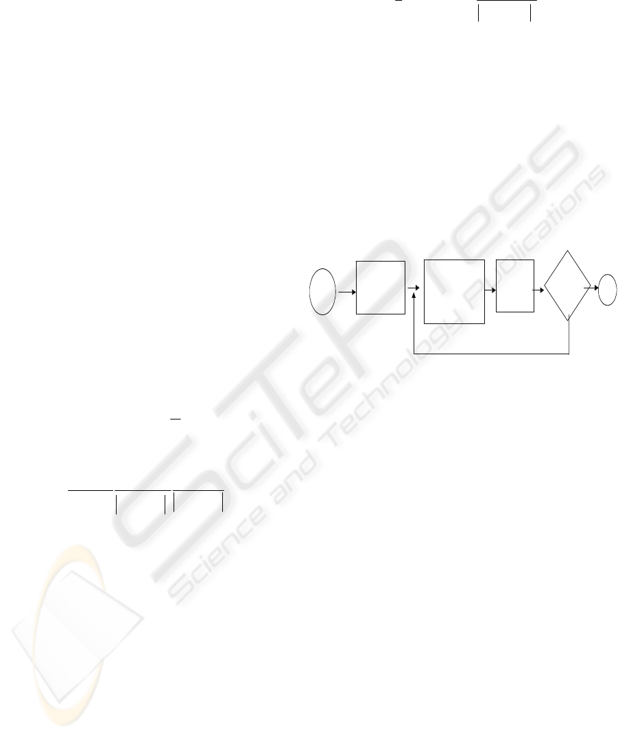
This section explains segmentation using
gravitational clustering in color space taking
neighbor relationship into account. The
segmentation proceeds as in figure 1.
Input
image
Mappi ng t o
Col or space
Upd a t e
nei ghbor r e l at i ons
i n c ol or space
gr avi t at i onal l
clustering
Any c hanges
in
Clusters
?
?
st op
yes
no
Figure 1: The configuration of segmentation process
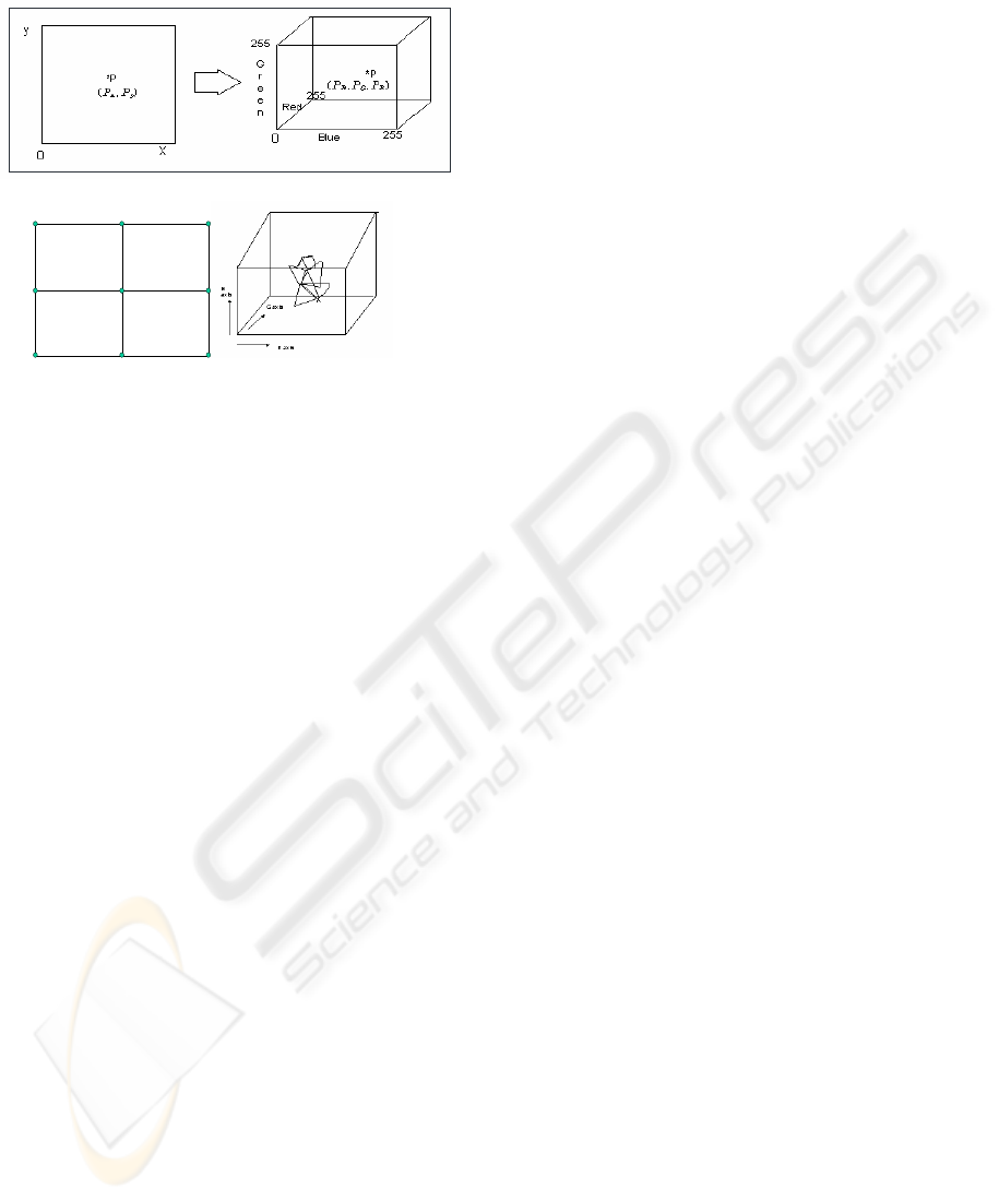
3.1 Mapping an image into the color
space
This section explains the mapping of pixels in an
image into color space. A pixel of (R, G, B) image
can be considered as a 5-tuple (r,g,b,x,y). Most
measurement space techniques uses only the
distances in (R, G, B) color space ignoring (x,y).
However, we use both (r,g,b) and (x,y) in the
clustering. As the two sources of information are of
different units, we should treat them differently:
(r,g,b) is used to compute distance as in other
algorithms, and location information (x,y) is
incorporated in neighbor relations along which the
clustering process is performed. Figure 2 shows that
a pixel
P
at (
yx
) with (R,G,B) value
(
BGR
) is mapped to
PP ,
PPP ,,
'
P
at (
BGR
) in
(R,G,B) space. Most measurement space algorithms
use only (
BGR
) in (R,G,B) space and ignore
spatial information (
y
).Figure 3(a) shows an
image region of 3
PPP ,,
PPP ,,
x
PP ,
×
3 pixels connected by 4-
neighbor relationship in the spatial domain. Figure
3(b) conceptually shows how those pixels map to
color space with their neighbor relations kept as
lines. In the clustering stage, we apply gravitational
force only among neighboring pixels . That is, even
if two pixels may be close to each other in color
COLOR IMAGE SEGMENTATION BY GRAVITATIONAL CLUSTERING IN COLOR SPACE USING
NEIGHBOR-RELATIONSHIP
271

space, they would not attract each other unless they
are spatial neighbors.
Figure 2: Mapping of a pixel
(a) 3×3 pixels in special domain connected by 4-neighbor
(b) specially neiboring pixels in color space
Figure 3: Pixels in spatial domain and in color space
3.2 Gravitational clustering utilizing
neighbour relations
As stated above, those pixels close to each other in
color space are clustered only if they are connected
by neighbor relations, not like other measurement
space algorithms such as (Yung, 1998). The
algorithm is as follows:
Step 1. Let each pixel be a particle.
Initialize parameters such as merging distance
ε
.
Step 2. Update neighbor relations altered by merged
particles
(Initially 8-neighbor).
Step 3. Compute gravitational force among
neighbors, move particles in color space according
to the gravitational force attraction.
Step 4. If the distance to a neighbor is less than
ε
,
merge it with the neighbor.
Step 5. If there is no more merge or movement of
particles, then stop.
Otherwise, go to step 2.
The Markov model discussed in section 2.1 is used
in step 3. The resulting particles are clusters, and
pixels in each cluster belong to a segment.
3.2.1 The merging distance
ε
The
ε
can be determined in many ways; we
considered the distance histogram which
accumulates distances between a pixel and its
neighbors in color space. Pixels in a segment have
similar color value, making a high peak near
distance zero in the histogram. The first valley of the
histogram where the histogram value starts
increasing after the decrease from the high peak near
zero distance can be a candidate for the
ε
value.
However, if
ε
is too small, the image may be over-
segmented. Thus, we selected the first valley beyond
a distance of 10 from the zero peak that is
empirically obtained. In most cases, a value of 16
produced good results. As clustering proceeds, those
neighboring clusters having similar colors are
merged, and their centers are replaced by the center
of mass. Thus, the inter-cluster distances get bigger,
while intra-cluster distances get smaller. If
ε
is
large, the color error given in equation (5) of section
4 becomes large as the center value does not
represent the pixel values in the segment accurately,
but it will produce a small number of segments. If a
small
ε
is used, the image may be over-segmented
even if the error gets smaller.
3.2.2 Extent of gravitation effect
If the process of gravitational clustering is
continued, all the particles will be merged to form a
single cluster eventually. We need some provision to
prevent this and find optimal clusters. Various
methods taken by others are reviewed first.
Wright(Wright, 1977) applied the gravitational force
to all the data at all times. The clustering process
was actually continued until all the particles were
merged, and the time was measured between every
merge event and the next. The best clustering is
considered to be the clustered state just before the
longest time elapse until anothermerge event occurs.
This method has the disadvantage of long computing
time since the process must be continued until all the
particles are merged.
Yung and Lai(Yung, 1998) took a different approach.
They restricted the extent of gravitational force; they
called it “force effective field (FEF)”, conceptually
similar to the neighbor function of the SOFM neural
net(Kohonen, 1997). They decreased the extent of
FEF as the iteration proceeded.
Another possible method is to let the data space
expand like the Universe and find the equilibrium
state of contraction and expansion.
The approach taken in this paper is to restrict the
merge distance such that particles are merged only
when they are within a certain distance, and the
gravitational force is applied only to ‘neighboring’
particles in the spatial domain..
Figure 4 shows how the neighbor relation is updated
after a merge event. In the figure, p0….p6 are
particles (clusters) in the color space. The lines
represent neighbor relations and their lengths
represent the distances. Consider p0 for example.
The gravitational forces on p0 by p1,p2,p3 and p4
are computed; if p0 and p4 are merged together, new
neighbors of p0 are p1,p2,p3 and p5,p6 which were
ICINCO 2005 - SIGNAL PROCESSING, SYSTEMS MODELING AND CONTROL
272

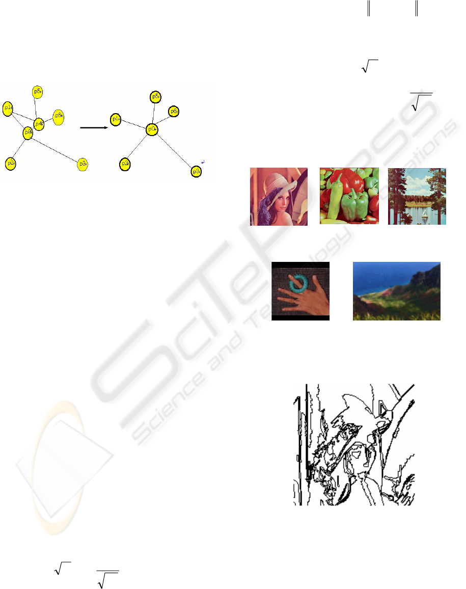
neighbors of p4 previously, as shown in figure 4(b).
In the next iteration, p0 would be affected by these
new neighbors. As two particles p0 and p4 are
merged, their mass becomes 2. Heavier particles will
exert stronger gravitational force than lighter ones,
and they will attract lighter ones toward them. This
effect is equivalent to finding the center of mass for
those pixels that belong to the cluster. As the
iteration continues, the number of particles will be
reduced by merging.
(a) before merge (b)after merge
Figure 4: Updating neighbor relations
3.3 Image Segmentation
Those algorithms that just find clusters in the color
space without considering neighbor relations need a
region labeling process after clustering to find
individual segments, since those clusters contain
pixels of similar color regardless of their location. In
contrast, our algorithm does not need region
labeling, since each cluster contains only
neighboring pixels of similar color. Even though
pixels may have similar color in RGB space, they do
not belong to a cluster unless they are neighbors to
others. Thus, a cluster corresponds to a separate
region in our algorithm.
4 EXPERIMENTAL RESULTS
True-color images were used as input to the
segmentation algorithm. The 8-neighbor relation
was used in the clustering. Experiments were
performed to compare the effect of the distance
parameter
ε
and the effect of taking neighbor
relations into account. The algorithm was then
compared with segmentation by the K-means
clustering algorithm. The following criterion (Liu,
1994) is used to measure the performance of
segmentation algorithms,
∑
=
×=
R
i
i
i
A
e
RIF
1
2
)(
(5)
where R is the number of regions,
is the
number of pixels in i-th region,
is color error of i-
th region defined as
i
A
i
e
∑
∈
−=
i
Ryx
yxyxi
ppe
),(
'
,,
. is
the original color value (r,g,b) of pixel at (x,y), and
is the color value of the segment to which the
pixel at (x,y) belongs. The
yx
p
,
'
, yx
p
R
factor imposes a
penalty for too many regions, and the
i
i
A
e
2
term
imposes a penalty for small regions or regions for
which the color difference error is large.
A smaller F value means better segmentation. We
normalized F with respect to image size.
a) Lena (b) pepper (c) sail boat
(160X160) (200X200) (128X128)
(d) hand (e) valley
(128×128) (96×64)
Figure 5: Images used in the experiments
(a) 20
COLOR IMAGE SEGMENTATION BY GRAVITATIONAL CLUSTERING IN COLOR SPACE USING
NEIGHBOR-RELATIONSHIP
273

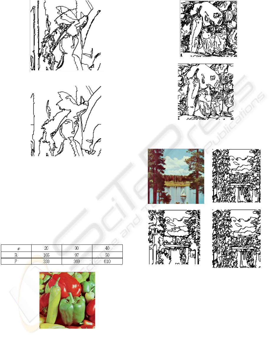
(b) 30
(c) 40
Figure 6: Variations on
ε
Figure 6 shows the results of varying
ε
. As
expected, a large value of
ε
produces a small
number of regions, while a small value of
ε
generates more regions. Thus, the value of
ε
can be
used for controlling the degree of details in
segmentation.
Table 1: The number of regions
(R) and evaluation (F) of results in figure.
(a) Original image
(b) K- means
(c) Proposed method
Figure 7: Comparison of K-means and our method for the
image in figure 5(b)
(a) Original image (b) K-means
(c)Gravitational
clustering
with neighbor relations
(d) gravitational
clustering without neighbor
relations
Figure 8: The K-means and gravitational clustering
algorithms with and without using neighbor relations for
the image in figure 5(c)
ICINCO 2005 - SIGNAL PROCESSING, SYSTEMS MODELING AND CONTROL
274

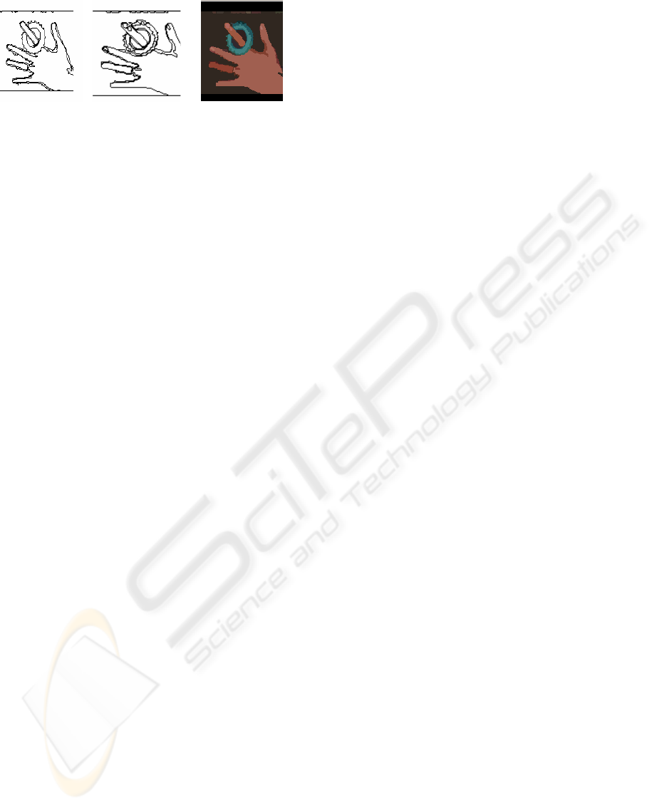
Figure 9: Another comparison of K-means and our
method
As we can see in the figure 7 and 8, the result of the
K-means method is not as good as our method for
images where the K (the number of color clusters)
is not easily given. In figure 9(c), each region is
painted with the center value of each cluster. It
shows that the upper part of the finger with the
smaller ring is separated from the other part of the
hand. This shows a characteristic of the proposed
algorithm, which separates regions that are not
adjacent even though their colors are similar. One
part of the finger is painted darker because fewer
pixels than the other part of the hand are contained
in the cluster and that part is more affected by
shadows . The K-means method in figure 9(a) does
not separate fingernails which may be important in
further image computations, and does not separate
darker protrusions on the larger ring. We compared
the gravitational clustering segmentation with and
without neighbor relations. By computing
gravitational force and allowing mergers for only
neighboring particles, the amount of computation is
greatly reduced and the speed is order of magnitude
faster compared to the algorithm without
incorporating the neighbor relations(Yung, 1998).
Proposed method also produced better segmentation
results in quality.
5 CONCLUSION
In this paper, a new segmentation algorithm is
proposed, which uses gravitational clustering in the
color space and incorporates neighbor relations. The
method produces better results compared to the K-
means method. As the clustering is performed along
the neighbor relations, pixels having similar colors
are not clustered unless they are adjacent. Hence
there is less need of a region labeling process.
Incorporation of neighbor relations also reduces the
computation time. As both the distance in the color
space and neighbor relations in the spatial domain
are used, it can be considered a hybrid of
measurement space and image space algorithms.
REFERENCES
(a) K-means (b) Proposed
method
(c) Result in (b)
painted with cluster
center values
Song Chun Zhu and Alan Yuille, 1995. Region
Competition: Unifying Snakes, Region Growing, and
Bayes/MDL for Multiband Image Segmentation. In
IEEE PAMI, vol. 18, No.9, pp. 884-900.
R. L. Cannon, J. V. Dave, and J. C. Bezdek, 1986.
Efficient Implementation of the Fuzzy c-Means
Clustering Algorithms. In IEEE PAMI, vol. 8, no. 2,
pp. 248-255.
Young Won Lim and Sang Uk Lee, 1990. On the Color
Image Segmentation Algorithm based on the
Thresholding and the Fuzzy c-Means Techniques. In
Pattern Recognition, vol. 23, no. 9, pp. 935-952.
H. C. Yung and H. S. Lai, 1998. Segmentation of color
based on the gravitational clustering concept. In
Optical Engineering, vol. 37, no. 3.
W. E. Wright, 1977. Gravitational Clustering. In Pattern
Recognition, vol. 9, pp.151-166.
Jianqing Liu and Yee-Hong Yang, 1994. Multiresolution
Color Image Segmentation. In IEEE PAMI, vol. 16,
no.7, pp. 689-700.
D. A. Forsyth, 2002. Computer Vision: A Modern
Approach, Prentice-Hall.
T. Kohonen, 1997. Self-Organizing Maps, Springer-
Verlag. 2nd edition.
COLOR IMAGE SEGMENTATION BY GRAVITATIONAL CLUSTERING IN COLOR SPACE USING
NEIGHBOR-RELATIONSHIP
275