
CONTROL OF DISCRETE LINEAR REPETITIVE PROCESSES
WITH VARIABLE PARAMETER UNCERTAINTY
B. Cichy
∗
∗
Institute of Control and Computation Engineering, University of Zielona G
´
ora
ul. Podg
´
orna 50, 65-246 Zielona G
´
ora, Poland
K. Gałkowski
∗, †
and A. Kummert
‡
†,‡
Bergische Universit
¨
at Wuppertal
Rainer-Gruenter-Strasse 21, D-42119 Wuppertal, Germany
E. Rogers
§
§
School of Electronics and Computer Science
University of Southampton, Southampton SO17 1BJ, UK
Keywords:
Controller design, variable uncertainty, robust control, LMI.
Abstract:
This paper is devoted to solving the problem of stabilising an uncertain discrete linear repetitive process, where
the model uncertainty is a result of the variable along the pass uncertainty of the parameters. The analysis is
applied to the engineering example of the material rolling process, which can be modelled as a repetitive
process (Rogers and Owens, 1992; Gałkowski et al., 2003b). Due to its analytical simplicity and due to
computational effectiveness, the LMI based approach to design a robust state controller for 2D systems has
been used here.
1 INTRODUCTION
Repetitive processes are a distinct class of 2D systems
of both system theoretic and applications interest.
The essential unique characteristic of such a process
is a series of sweeps, termed passes, through a set of
dynamics defined over a fixed finite duration known
as the pass length. On each pass an output, termed the
pass profile, is produced which acts as a forcing func-
tion on, and hence contributes to, the dynamics of the
next pass profile. This, in turn, leads to the unique
control problem for these processes in that the output
sequence of pass profiles generated can contain oscil-
lations that increase in amplitude in the pass-to-pass
direction.
The analysis of linear repetitive processes has re-
ceived considerable attention in the literature — see,
for example, (Rogers et al., 2005; Gałkowski and
Wood, 2001; Roberts, 2000; Rogers and Owens,
1992). Although these processes are well known,
many control design problems for them are still (rel-
∗
This work is partially supported by State /Poland/ Com-
mittee for Scientific Research, Grant no. 3 T11A 008 26.
†
K. Gałkowski is currently a Gerhard Mercator Guest
Professor in the University of Wuppertal
atively) open. This stems from the fact that control
of these processes using standard (or 1D) systems
theory/algorithms fails (except in a few very restric-
tive special cases) precisely because such an approach
ignores their inherent 2D systems structure, i.e. in-
formation propagation occurs from pass-to-pass and
along a given pass, and also the pass initial conditions
are reset before the start of each new pass.
Material rolling is one of a number of physically
based problems which can be modelled as a linear
repetitive process (Rogers and Owens, 1992). In this
paper, we use material rolling as a basis to illustrate
numerically algorithms the solution we develop to a
currently open robust stability and stabilization prob-
lem for the underlying sub-class of so-called discrete
linear repetitive processes. The design itself can be
executed in terms of a linear matrix inequality (LMI)
which, in turn, can be solved with well established
effective numerical algorithms (Gahinet et al., 1995;
Nesterov and Nemirovskii, 1994).
Inn physical applications, the system or process
parameters are most often not known exactly and
only some nominal values or admissible intervals are
available. Hence, although the nominal process is
most often time invariant, the uncertain process can
be time variant. This will be the case here and to
37
Cichy B., Gałkowski K., Kummert A. and Rogers E. (2005).
CONTROL OF DISCRETE LINEAR REPETITIVE PROCESSES WITH VARIABLE PARAMETER UNCERTAINTY.
In Proceedings of the Second International Conference on Informatics in Control, Automation and Robotics - Robotics and Automation, pages 37-42
DOI: 10.5220/0001161500370042
Copyright
c
SciTePress

solve the problem we generalize previously reported
LMI based design algorithms for uncertain repetitive
processes (Gałkowski et al., 2002) and other classes
of systems (Daafouz and Bernussou, 2001) with poly-
topic uncertainty. As the resulting solution requires
the presence of a convex uncertainty admissible set,
the question then arises as to what can be done in
cases where this is not true. Here we propose a so-
lution to this problem by first obtaining the convex
hull of the original non-convex uncertainty set.
Throughout this paper, the null matrix and the iden-
tity matrix with appropriate dimensions are denoted
by 0 and I, respectively. Moreover, a matrix, say
M < which is real symmetric and positive definite
is denoted by M > 0.
2 MATERIAL ROLLING AS
A LINEAR REPETITIVE
PROCESS
Material rolling is an extremely common industrial
process where, in essence, deformation of the work-
piece takes place between two rolls with parallel axes
revolving in opposite directions.
In practice, a number of models of this process can
be developed depending on the assumptions made on
the underlying dynamics and the particular mode of
operation under consideration. Here, we restrict at-
tention to a linearised model of the dynamics. In
particular, following, for example (Gałkowski et al.,
2003b), the model considered is a so-called discrete
linear repetitive process whose state space model is
of the form
x
k+1
(p + 1) = Ax
k+1
(p) + Bu
k+1
(p) + B
0
y
k
(p) (1)
y
k+1
(p) = Cx
k+1
(p) + Du
k+1
(p) + D
0
y
k
(p)
Here on pass k, x
k
(p) ∈ R
n
is the state vector,
y
k
(p) ∈ R
m
is the pass profile vector, u
k
(p) ∈ R
l
is the vector of control inputs. To detail the structure
for our material rolling example, first introduce
u
k+1
(p)=F
M
(p)
x
k+1
(p)=
y
k+1
(p−1) y
k+1
(p−2) y
k
(p−1) y
k
(p−2)
T
A=
a
1
a
2
a
4
a
5
1 0 0 0
0 0 0 0
0 0 1 0
B=
b
0
0
0
B
0
=
a
3
0
1
0
(2)
C=
a
1
a
2
a
4
a
5
D= b D
0
= a
3
where
a
1
=
2M
λT
2
+M
a
2
=
−M
λ
2
T +M
a
3
=
λ
λT
2
+M
T
2
+
M
λ
1
a
4
=
−2λM
λ
1
(λT
2
+M)
a
5
=
λM
λ
1
(λT
2
+M)
b =
−λT
2
λ
2
(λT
2
+M)
The systems variables in above expressions are:
y
k+1
(p) and y
k
(p), which denote thickness of the ma-
terial on the current and previous pass respectively,
M is the lumped mass of the roll-gap adjusting mech-
anism, λ
1
is the stiffness of the adjustment mecha-
nism spring, λ
2
is the hardness of the material strip,
λ =
λ
1
λ
2
λ
1
+λ
2
is the composite stiffness of the material
strip and the roll mechanism. Finally, F
M
(p) is the
force developed by the motor and T is the sampling
period.
To complete the process description it is necessary
to specify the pass length and the initial, or boundary,
conditions, i.e. the pass state initial vector sequence
and the initial pass profile. Here these are taken to be
of the form
x
k+1
(0) = d
k+1
, k ≥ 0
y
0
(p) = f (p), 0 ≤ p ≤ α − 1 (3)
where d
k+1
is an n × 1 vector with constant entries
and f(p) is an m × 1 vector whose entries are known
functions of p. For ease of presentation, we make
no further explicit reference to the boundary condi-
tions except in Section 5 where a numerical example
is given.
3 STABILITY AND
STABILIZATION OF DISCRETE
LINEAR REPETITIVE
PROCESSES
The stability theory (Rogers and Owens, 1992) for
linear repetitive processes consists of two distinct
concepts but here it is the strongest of these, termed
stability along the pass, which is of interest. In
essence, this property (recall the unique control prob-
lem for these processes) demands bounded-input
bounded-output stability (defined in terms of the norm
on the underlying function space) uniformly, i.e. in-
dependent of the pass length. Several sets of neces-
sary and sufficient conditions for its existence but in
this paper it is the following result which is the start-
ing point. Even though this condition is sufficient but
not necessary, it forms a basis for control law design,
a feature which is not present in currently available
necessary and sufficient conditions.
Theorem 1 (Gałkowski et al., 2003a) A discrete lin-
ear repetitive process described by (1) is stable along
the pass if ∃ matrices W
1
> 0 and W
2
> 0 such that
the Lyapunov inequality
A
T
W A − W < 0 (4)
holds and W = diag {W
1
, W
2
} > 0, where
A =
A B
0
C D
0
(5)
ICINCO 2005 - ROBOTICS AND AUTOMATION
38
To provide a Lyaunov interpretation of this result
(which will be used extensively in the analysis to fol-
low in this paper), introduce the candidate Lyapunov
function as
V(k, p) = x
T
k+1
(p)W
1
x
k+1
(p) + y
T
k
(p)W
2
y
k
(p) (6)
where W
1
> 0, W
2
> 0, with associated increment
∆V(k, p) = x
T
k+1
(p + 1)W
1
x
k+1
(p + 1) + y
T
k+1
(p)W
2
y
k+1
(p) − x
T
k+1
(p)W
1
x
k+1
(p) − y
T
k
(p)W
2
y
k
(p). (7)
Then it is easy to show that
∆V(k, p) < 0 (8)
is equivalent to (4). For this reason, and the quadratic
structure of the Lyapunov function, stability along the
pass is also referred to as quadratic stability.
An extensively analyzed control law for the
processes considered here has the following form over
0 ≤ p ≤ α − 1, k ≥ 0
u
k
(p + 1) =
K
1
K
2
x
k
(p)
y
k−1
(p)
(9)
where K
1
and K
2
are appropriately dimensioned ma-
trices to be designed. In effect, this control law is
composed of the weighted sum of current pass state
feedback and feedforward of the previous pass pro-
file.
The LMI of (4) extends in a natural manner to the
design of (9) for stability along the pass (or quadratic
stability), but here we will use the approach based
on (Peaucelle et al., 2000) and first adopted for repet-
itive processes in (Gałkowski et al., 2003a). This will
prove to be of particular use in the analysis of the case
when there is uncertainty in the model.
Theorem 2 (Gałkowski et al., 2003a) Suppose that
a control law of the form (9) is applied to a discrete
linear repetitive process of the form described by (1).
Then the resulting process is stable along the pass if
∃ matrices W = diag {W
1
, W
2
}, W
1
> 0, W
2
> 0,
G = diag {G
1
, G
2
}, and N = diag {N
1
, N
2
}, such
that
−G − G
T
+ W (AG + BN )
T
AG + BN −W
< 0 (10)
If this condition holds, stabilizing K
1
and K
2
in the
control law (9) are given by K = N G
−1
, where K =
diag{K
1
, K
2
} and
b
B is given by
B = diag {B, D} (11)
4 ROBUST STABILITY AND
STABILIZATION OF DISCRETE
LINEAR REPETITIVE
PROCESSES
The design of control laws for discrete linear repeti-
tive processes has been the subject of much research
effort (Gałkowski et al., 2003b; Gałkowski et al.,
2003a; Gałkowski et al., 2002) and here we continue
the development of this general area by giving new re-
sults relating to the practical case when there is uncer-
tainty associated with the process (state space model)
description. In particular, we consider the case when
the model matrices
b
A,
b
B
are not precisely known,
but belong to a convex bounded (polytope type) un-
certain domain D. This, in turn, means that any un-
certain matrix can be written as a convex combination
of the vertices of the polytope D defined as follows
D =
A(ξ(k, p)), B(ξ(k, p)) : A(ξ(k, p)),
B(ξ(k, p)) =
v
i=1
ξ
i
(k , p)
A
i
, B
i
;
v
i=1
ξ
i
(k , p ) = 1;
ξ
i
(k , p) ≥ 0; k ≥ 0; 0 ≤ p ≤ α − 1
(12)
where v denotes the number of vertices. Note also
that the uncertainty here is variable in both indepen-
dent directions of information propagation, i.e. along
the pass (depends on p) and pass-to-pass (depends
on k).
Now we can write the following linear parameter
dependent system describing the process dynamics
x
k+1
(p + 1) = A
ξ(k, p) x
k+1
(p) + B ξ(k, p) u
k+1
(p)
+ B
0
ξ(k, p) y
k
(p)
y
k+1
(p) = C ξ(k, p) x
k+1
(p) + D ξ(k, p) u
k+1
(p)
+ D
0
ξ(k, p) y
k
(p) (13)
and also the parameterized candidate Lyapunov func-
tion
V(k, p, ξ(k, p)) = x
T
k+1
(p)
T
W
1
(ξ(k, p))x
k+1
(p)
+ y
T
k
(p)W
2
(ξ(k, p))y
k
(p) (14)
with
W
1
(ξ(k, p)) =
v
i=1
ξ
i
(k , p )W
1i
W
2
(ξ(k, p)) =
v
i=1
ξ
i
(k , p )W
2i
(15)
Also V(0, 0, ξ(0, 0)) < ∞ and the Lyapunov func-
tion increment is given by
∆V(k, p, ξ(k, p)) = x
T
k+1
(p + 1)W
1
ξ(k, p + 1)
x
k+1
(p+1)+y
T
k+1
(p)W
2
ξ(k+1, p) y
k+1
(p)−x
T
k+1
(p)
W
1
ξ(k, p) x
k+1
(p) − y
T
k
(p)W
2
ξ(k, p) y
k
(p) (16)
Hence we can define the so-called poly-quadratic
stability for the repetitive processes considered here
(see (Daafouz and Bernussou, 2001) for the 1D sys-
tems case).
Definition 1 A discrete linear repetitive process de-
scribed by (1) with uncertainty defined by (12) is said
to be poly-quadratically stable provided
∆V
k, p, ξ(k, p) < 0 (17)
∀ k ≥ 0, 0 ≤ p ≤ α − 1
CONTROL OF DISCRETE LINEAR REPETITIVE PROCESSES WITH VARIABLE PARAMETER UNCERTAINTY
39

The requirement of (17) is easy seen to be equiva-
lent to
A ξ(k, p )
T
diag
W
1
ξ(k, p + 1) , W
2
ξ(k + 1, p)
A ξ(k, p) − diag W
1
ξ(k, p) , W
2
ξ(k, p) < 0
(18)
where
b
A of (5) now becomes
A ξ(k, p) =
A ξ(k, p ) B
0
ξ(k, p)
C ξ(k, p) D
0
ξ(k, p)
=
v
i=1
ξ
i
(k , p )
A
i
(19)
and
b
A
i
is a polytope vertex, see (12).
Remark 1 When diag{W
1
ξ(k, p + 1) , W
2
ξ(k +
1, p)
} = diag{W
1
ξ(k, p) , W
2
ξ(k, p) } = W then
poly-quadratic stability reduces to quadratic stability
as in Corollary 1.
Now we have the following result from (Cichy
et al., 2005) which (drawing on the work in (Daafouz
and Bernussou, 2001)) aims to minimize the conser-
vativeness present from the use of a sufficient but not
necessary stability condition.
Theorem 3 A discrete linear repetitive process of the
form described by (1) with uncertainty defined by (12)
is poly-quadratically stable if ∃ block diagonal matri-
ces
b
S
i
, i = 1, 2, . . . , v, i.e.
b
S
i
= diag {S
i1
, S
i2
}, and
matrices
b
G = diag {G
1
, G
2
} such that
G + G
T
− S
i
G
T
A
T
i
A
i
G S
j
> 0 (20)
for all i, j = 1, 2, . . . , v.
With the control law (9) applied, (20) becomes
G + G
T
− S
i
G
T
(A
i
+ B
i
K)
T
(
A
i
+ B
i
K)G S
j
> 0 (21)
where K = diag {K
1
, K
2
}. The following re-
sult now gives a sufficient condition for the existence
of a poly-quadratically stabilizing control law of the
form (9) for the case under consideration.
Theorem 4 Suppose that a control law of the
form (9) is applied to a discrete linear repeti-
tive process described by (1) with uncertainty de-
fined by (12). Then the resulting process is poly-
quadratically stabilizable if ∃ symmetric matrices
b
S
i
> 0, i = 1, 2, . . . , v, i.e.
b
S
i
= diag {S
i1
, S
i2
}
and
b
G = diag {G
1
, G
2
},
b
N = diag {N
1
, N
2
}, such
that the following LMI is feasible
G + G
T
− S
i
G
T
A
T
i
+ N
T
B
T
i
A
i
G + B
i
N S
j
> 0 (22)
for all i, j = 1, . . . , v. If this condition holds then
stabilizing K
1
and K
2
in the control law are given by
(9) with
K =
NG
−1
(23)
where K = diag {K
1
, K
2
} .
Proof: Follows immediately from (21) on setting
K
b
G =
b
N.
5 APPLICATION TO THE
MATERIAL ROLLING
EXAMPLE
In this section we apply our new design to the material
rolling model of Section 2 when the model parameters
T, M, λ
1
, λ
2
are uncertain. In order to avoid a control
law with very large entries in the defining matrices,
we limit attention to solutions of the LMI (22) where
the matrix N is diagonal. The boundary conditions
are x
k+1
(p) = 0, k ≥ 0 and y
0
(p) = 1, 0 ≤ p ≤
14, and in the simulations given below x
1
k
(p) denotes
the first entry of the state vector x
k
(p), the number of
passes is 26, and the number of points along the pass
is 15.
Consider first the case when the discretization pe-
riod belongs to the interval
T ∈ [T
, T ] = [0.21, 0.25] (24)
and the rest of parameters satisfy
M ∈ [M , M ] = [90, 110], λ
1
∈ [λ
1
, λ
1
] = [430, 600]
λ
2
∈ [λ
2
, λ
2
] = [1970, 2070]. (25)
Here the uncertainty domain has 16 vertices, but is
not convex and hence the new design procedure de-
veloped in this paper cannot be applied. To overcome
this difficulty, we first use the Geometric Bounding
Toolbox (GBT) to numerically estimate the minimum
convex domain (i.e. convex hull) which covers the
original non-convex one. (This, of course, introduces
extra conservativeness.)
The resulting convex domain which now be
used to execute our new design algorithm for the
example considered has the following 6 vertices
Vertex 1
A =
1.7502 −0.0041151 −1.4491 0.72457
1 0 0 0
0 0 0 0
0 0 1 0
C =
1.7502 −0.0041151 −1.4491 0.72457
B =
−6.0343e − 5
0
0
0
B
0
=
0.84948
0
1
0
D = −6.0343e − 5 D
0
= 0.84948
Vertex 2
A =
1.5159 −0.001699 −1.162 0.58098
∗
C =
1.5159 −0.001699 −1.162 0.58098
B =
−0.00012288
∗
B
0
=
0.82305
∗
D = −0.00012288 D
0
= 0.82305
ICINCO 2005 - ROBOTICS AND AUTOMATION
40
Vertex 3
A =
1.6886 −0.0024702 −1.2944 0.6472
∗
C =
1.6886 −0.0024702 −1.2944 0.6472
B =
−7.9026e − 5
∗
B
0
=
0.80288
∗
D = −7.9026e − 5 D
0
= 0.80288
Vertex 4
A =
1.6035 −0.0028319 −1.3277 0.66386
∗
C =
1.6035 −0.0028319 −1.3277 0.66386
B =
−9.5766e − 5
∗
B
0
=
0.8621
∗
D = −9.5766e − 5 D
0
= 0.8621
Vertex 5
A =
1.5117 −0.001661 −1.172 0.58599
∗
C =
1.5117 −0.001661 −1.172 0.58599
B =
−0.00011795
∗
B
0
=
0.83015
∗
D = −0.00011795 D
0
= 0.83015
Vertex 6
A =
1.5159 −0.001699 −1.162 0.58098
∗
C =
1.5159 −0.001699 −1.162 0.58098
B =
−0.00012288
∗
B
0
=
0.82305
∗
D = −0.00012288 D
0
= 0.82305
where ∗ denotes an entry equal to that of the corre-
sponding value for Vertex 1.
The parameters T, M, λ
1
, λ
2
vary on each
pass k stochastically with p within the con-
stant intervals (24) and (25) respectively and
are denoted by T (k, p), M (k, p), λ
1
(k, p), and
λ
2
(k, p) respectively. Note also that the functions
T (k, p), M (k, p), λ
1
(k, p), and λ
2
(k, p) can be
different on each pass k.
Applying Theorem 4 now gives the stabilizing con-
trol law matrices
K
1
=
18161.073 −31.212 −10010.633 7335.353
K
2
= 9425.674. (26)
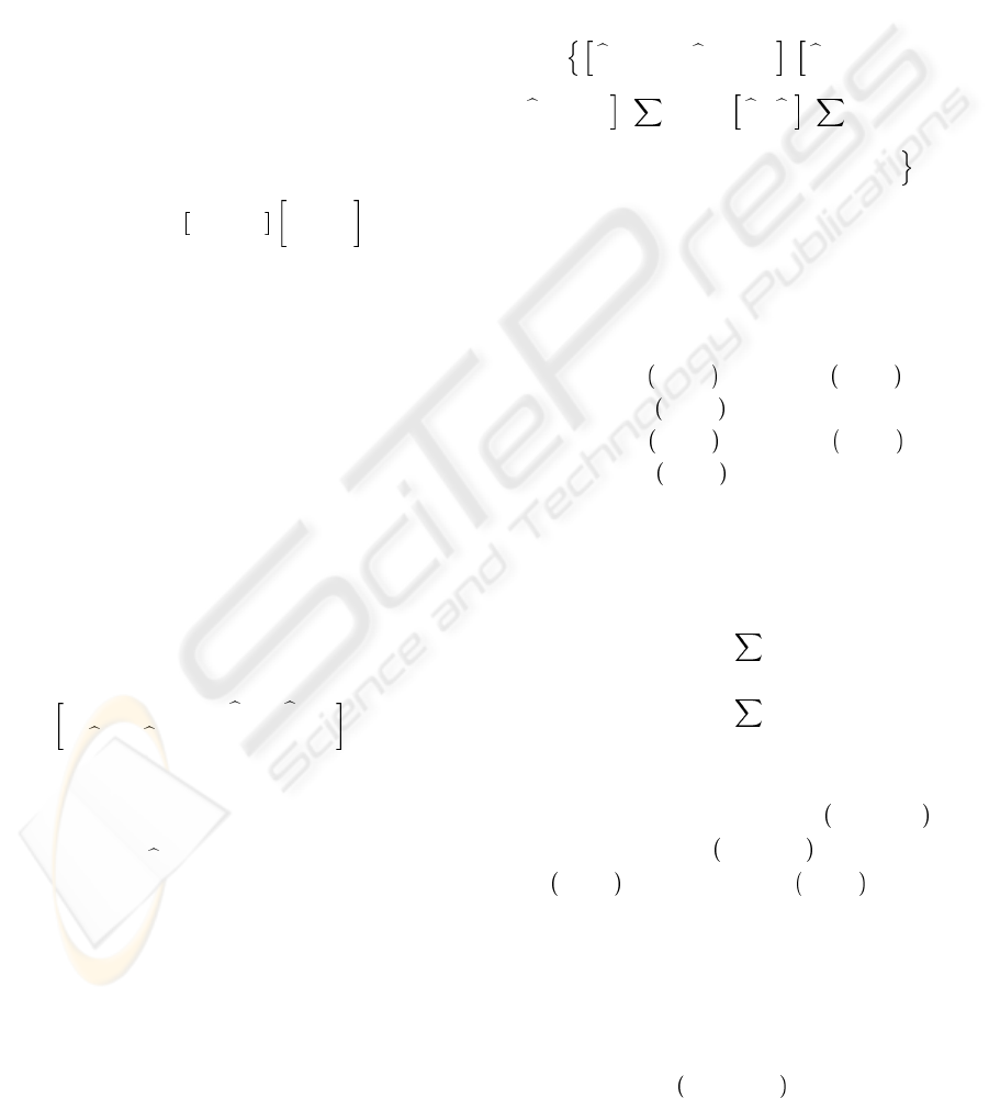
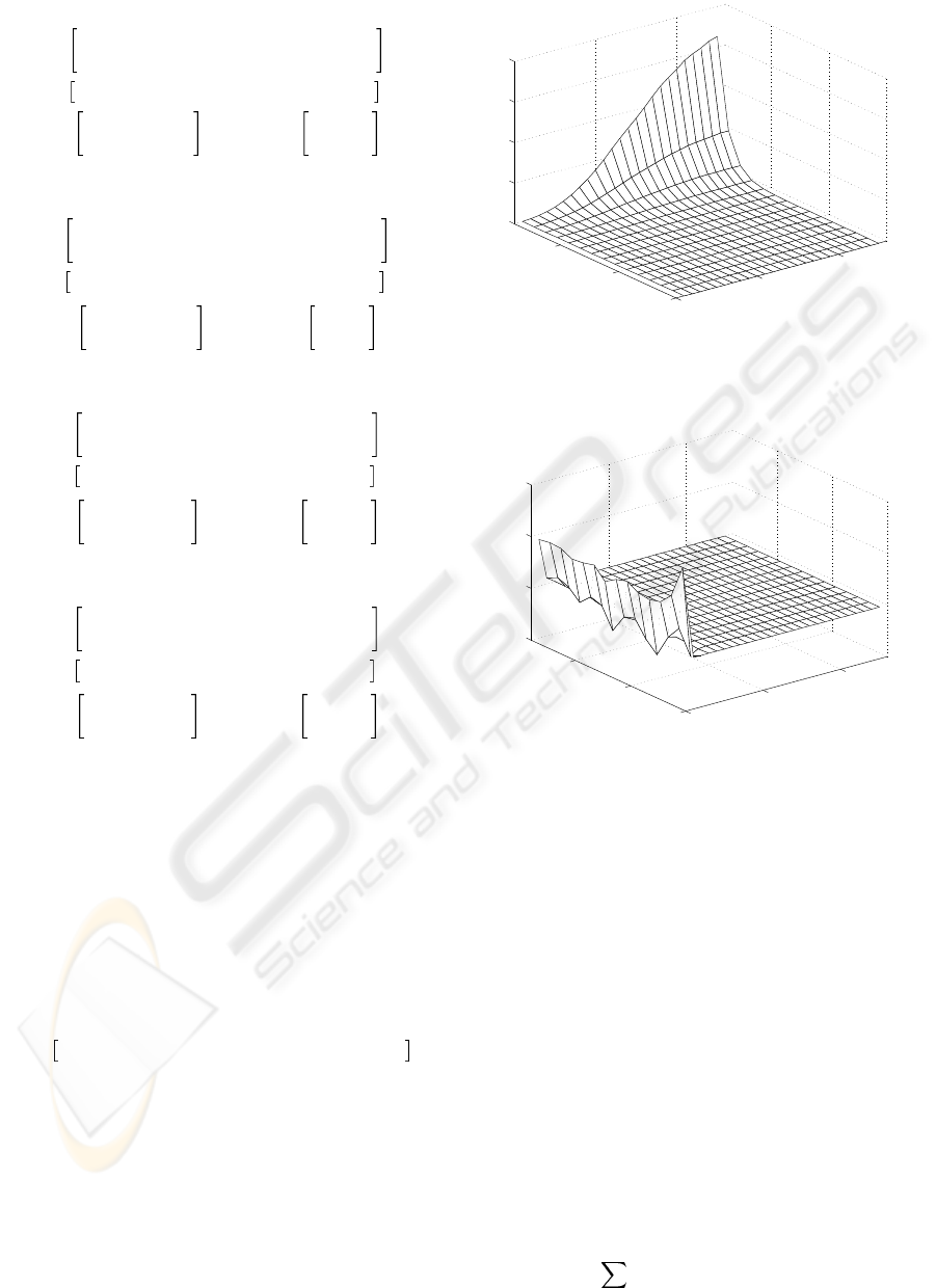
Figures 1 and 2 show the pass profile se-
quences generated by the uncontrolled and controlled
processes respectively (with zero input sequence).
To conclude this section, it is instructive to give
some comments on the steps necessary to apply the
new design algorithm developed in this paper. The
first point is that we have 4 parameters which can
vary between given maximum and minimum values
0
10
20
0
5
10
0
1
2
3
4
x 10
5
pass to pass
along the pass
Figure 1: The process pass profile sequence with no control
action applied (plot is x
1
k
(p)).
0
10
20
0
5
10
−0.5
0
0.5
1
pass to pass
along the pass
Figure 2: The process pass profile sequence with control
action applied (plot is x
1
k
(p)).
and hence there are 16 combinations for the uncer-
tainty domain vertices, and the uncertainty domain is
required to be convex. If, as in the numerical example
above, convexity is not present, then the most obvi-
ous idea is to numerically estimate the convex hull of
the vertices where here we have used (GBT). This,
of course, introduces extra conservativeness into the
design and how to reduce this is clearly a subject for
further research.
Suppose now that a control law has been success-
fully designed and we wish to simulate the response
of the process under control action. Then we first have
to determine ξ
i
(p) ∀i = 1, 2, . . . , v and 0 ≤ p ≤
α−1, where v denotes number of vertices. We can do
this by applying Matlab function fmincon to solve
the following problem: determine ξ
i
(k, p) ∈ R
+
,
i = 1, 2, . . . , v such that
v
i=1
ξ
i
(k , p)V
i
= P (k, p) (27)
CONTROL OF DISCRETE LINEAR REPETITIVE PROCESSES WITH VARIABLE PARAMETER UNCERTAINTY
41

where
v
i=1
ξ
i
(k , p) = 1; ξ
i
(k , p) ≥ 0;
k ≥ 0; 0 ≤ p ≤ α − 1
Here the V
i
denote the minimal convex domain ver-
tices and P (k, p) denotes a matrix within the obtained
polytope for point p on pass k, i.e the corresponding
process state space model matrix computed from the
corresponding T (k, p), M(k, p), λ
1
(k, p), λ
2
(k, p).
Repeating this procedure ∀ k ≥ 0 and ∀ p,
0 ≤ p ≤ α − 1, enables the process response with or
without control action applied
6 CONCLUSION
In this paper, we have extended previous results on
the stability and control of discrete linear repeti-
tive processes to the case when the defining state
space model matrices are subject polytopic uncer-
tainty. This has led to a design algorithm which can
be implemented using well tested software. Also we
have attempted to minimize the conservativeness in-
troduced by the use of sufficient only conditions for
stability.
REFERENCES
Cichy, B., Gałkowski, K., and Rogers, E. (2005). Control
of uncertain discrete linear repetitive processes based
on the physical example. Proceedings of 4th Interna-
tional Workshop On Multidimensional (ND) Systems,
Wuppertal, Germany (in press).
Daafouz, J. and Bernussou, J. (2001). Parameter depen-
dent lyapunov functions for discrete time systems with
time varying parametric uncertainties. Systems &
Control Letters, 43:355–359.
Gahinet, P., Nemirowski, A., Laub, A. J., and Chilali, M.
(1995). LMI Control Toolbox for use with MATLAB.
The Mathworks Partner Series. The MathWorks Inc.
Gałkowski, K., Lam, J., Rogers, E., Xu, S., Sulikowski, B.,
Paszke, W., and Owens, D. H. (2003a). LMI based
stability analisys and robust controller design for dis-
crete linear repetetive processes. International Jour-
nal of Robust and Nonlinear Control, 13:1195–1211.
Gałkowski, K., Rogers, E., Paszke, W., and Owens, D.
(2003b). Linear repetitive process control theory ap-
plied to a physical example. Applied Mathematics and
Computer Science, 13(1):87–99.
Gałkowski, K., Rogers, E., Xu, S., Lam, J., and Owens, D.
(2002). LMIs -a fundamental tool in analysis and con-
troller design for discrete linear repetitive processes.
IEEE Transactions on Circuits and Systems I, Funda-
mental Theory and Applications, 49(6):768–778.
Gałkowski, K. and Wood, J. (2001). Multidimensional Sig-
nals, Circuits and Systems. Taylor & Francis.
Nesterov, Y. and Nemirovskii, A. (1994). Interior-point
Polynomial Algorithms in Convex Programing, vol-
ume 13 of SIAM Studies in Applied Mathematics.
SIAM, Philadelphia.
Peaucelle, D., Arzelier, D., Bachelier, O., and Bernussou, J.
(2000). A new robust D-stability condition for poly-
topic uncertainty. Systems & Control Letters, 40:21–
30.
Roberts, P. D. (2000). Numerical investigations of a stabil-
ity theorem arising from 2-dimensional analysis of an
iterative optimal control algorithm. Multidimensional
Systems and Signal Processing, 11 (1/2):109–124.
Rogers, E., Gałkowski, K., and Owens, D. (2005). Control
Systems Theory and Applications for Linear Repeti-
tive Processes. Lecture Notes in Control and Informa-
tion Sciences. Springer-Verlag. (in print).
Rogers, E. and Owens, D. (1992). Stability Analysis for
Linear Repetitive Processes, volume 175 of Lecture
Notes in Control and Information Sciences. Springer-
Verlag.
ICINCO 2005 - ROBOTICS AND AUTOMATION
42
