A MODEL BASED CONTROL OF COMPRESSED NATURAL
GAS INJECTION SYSTEMS
Bruno Maione, Paolo Lino, Alessandro Rizzo
Dipartimento di Elettrotecnica ed Elettronica, Politecnico di Bari, via Re David 200, 70125 Bari, Italy
Keywords: Modeling injection systems, Common Rail, CNG, Pressure control.
Abstract: Low fuel consumption and low emissions are key issues in modern internal combustion engines design. For
this reason, an effective on-line control of the injection process requires the mathematical equations
describing the system dynamics. The inherent nonlinearities make the modeling of the fuel-injection system
hard to accomplish. Moreover, it is necessary to trade off between accuracy in representing the dynamical
behavior of the most significant variables and the need of reducing complexity to simplify the controller
design process. In this paper we present a second order lumped parameters model of a Compressed Natural
Gas injection system for control system synthesis and analysis. Based on the proposed model, we propose a
generalized predictive controller to regulate the injection pressure, which guarantees good performances and
robustness to modeling errors.
1 INTRODUCTION
Today it is a widely accepted opinion that
performances of internal combustion engines strictly
depend on fuel injection dynamics and metering of
air/fuel mixture (Heywood). Owing to a better
control on air/fuel ratio, the innovative Common
Rail injection system remarkably reduces noxious
emissions, consumptions and noise in Diesel
engines, while improving efficiency and available
power (Maione, 2004a). These goals are achieved by
setting the injection pressure to a fixed value, while
controlling injection timings electronically for
different operating conditions.
It is also well known that, if compared to liquid
fuels, t
he Compress Natural Gas (CNG) reduces
polluting emissions of CO, NOx, HC and particulate
of internal combustion engines, and guarantees their
better efficiency, thanks to its good antiknock
properties (Weaver). However, greater difficulties in
metering make the use of CNG less worthwhile.
This drawback can be overcome by applying the
Common Rail technology to CNG engines and by
using the injection control to improve performances.
However, improving the controllers design process
requires a quite accurate model for predicting the
system behavior.
Injection system models for Diesel
engines are
mainly based on three different approaches. The
straightest one is founded on fluid-dynamic
simulation packages like AMESIM, which
encompasses libraries of mechanical components,
and requires precise knowledge of the system
geometrical data (Mulemane). Although the
resulting models provide an accurate representation
of system dynamics, which is appropriate for
mechanical design, they are not in the form of
mathematical equations useful for control purposes.
Different classes of models descend from
identification processes based on real data. They
guarantee a good prediction of the system behavior
if nonlinear functions are exploited (Maione,
2004b). Finally, some injection system models are
based on equations describing the physics
underlying the process. Basically, this approach
leads to Partial Differential Equations or high order
representations, which are certainly not suitable for
control purposes (Cantore), (Kouremenos), (Maione,
2004a).
However, to the best authors knowledge, there is
lack
of studies carried out for modeling and
controlling gaseous fuel injection systems. In this
paper we propose a simple lumped parameters
model describing only main fluid-dynamic
phenomena of the CNG injection system. It is in the
form of a second order state space representation
suitable for designing controllers of the rail pressure.
Moreover, we also stress that tuning the parameters
of the model requires a minimal set of the system
geometric data. Finally, on the basis of this model
132
Maione B., Lino P. and Rizzo A. (2005).
A MODEL BASED CONTROL OF COMPRESSED NATURAL GAS INJECTION SYSTEMS.
In Proceedings of the Second International Conference on Informatics in Control, Automation and Robotics - Robotics and Automation, pages 132-137
DOI: 10.5220/0001158401320137
Copyright
c
 SciTePress

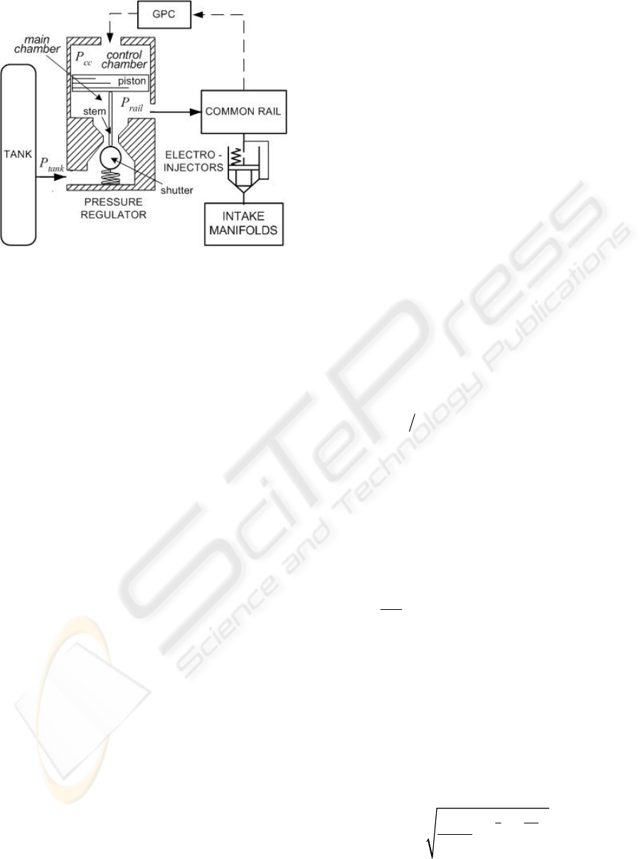
Figure 1: Block scheme of the CNG Common Rail
injection system
we show how to design a Generalized Predictive
Controller (GPC) for the rail pressure which
parameters directly descend from the model
equations (Rossiter).
2 STATE SPACE MODELING OF
THE CNG INJECTION SYSTEM
The main elements of the CNG injection system are
a fuel tank, storing high pressure gas, a controlled
pressure regulator, a common rail and four electro-
injectors. The regulator reduces the pressure of the
fuel supplied by a tank, and sends it to the common
rail, feeding the electronically controlled injectors.
Then the injectors send the gas to the intake
manifolds to obtain the proper air/fuel mixture
(Figure 1).
The large volume of the common rail helps in
damping the oscillations due to the operation of both
pressure regulator and injectors. So it ensures a
constant pressure as requested by a correct metering
of the injected fuel. In fact, the injection flow only
depends on rail pressure and injection timings,
which are precisely driven by the Electronic Control
Unit (ECU). The output signal of a pressure sensor
inside the rail is processed to close the control loop.
The pressure regulator consists of a main
chamber with a variable inflow section, which
depends on the axial displacement of a spherical
shutter over a conical seat, and of a control chamber,
whose pressure is regulated by a solenoid valve. A
piston between the two chambers provides the seal
for the main valve shutter. The equilibrium of the
applied forces determines piston and shutter
dynamics (Smith) (Figure 1). In particular, the
control chamber pressure is regulated by varying the
driving current duty cycle (d.c.) among a control
period, making the valve opened and closed in turn:
in this way is possible to control the fuel flow from
the tank towards the rail. Finally, to maintain an
equilibrium condition in steady state operation, the
fuel in the control chamber is sent to the main circuit
through an high resistance orifice.
To model the CNG injection system we consider
two control volumes having a uniform, time varying,
pressure distribution, i.e. the regulator control
chamber and the rail circuit. We consider the tank
pressure as an input rather than a state variable as its
measure is always available on board as it is related
to the fuel supply. Furthermore, it is likely to assume
equal injection and rail pressures, so that electro-
injectors are not modeled apart, but included in the
rail circuit as control electronic valves. Finally, we
assume a constant temperature in the whole injection
system, so that the system dynamics is completely
defined by the pressure variations in the control
chamber and the rail circuit.
Continuity equation and perfect gas law
(Zucrow) lead to the state equations of control
volumes. In particular the perfect gas law is:
pmRTV=
(1)
where p is the control volume pressure, R the gas
constant, T the temperature and m the fuel mass
stored in the instantaneous volume V. We can
neglect possible volume changes due to mechanical
part motions (for example in the control chamber)
without sensibly affecting the model accuracy.
Hence the derivative of (1), immediately gives the
continuity equation:
(
in out
RT
pmm
V
=−
&&&
)
(2)
where
in
and
out
are the input and output mass
flows, which sum has to be equal to the overall mass
change in the control volume. Integrating the
equation (2), after the evaluation of mass exchanges,
yields the pressure in the generic control volume.
m
&
m
&
By considering mass flows through control
chamber and regulator inlet orifices as isentropic
transformations and by applying momentum
equation, we get the following equations, depending
on the output/input pressure ratio r = p
o
/p
i
(Zucrow):
21
2
1
in d in
k
kk
kRT
mcA rr
k
ρ
+
=⋅−
−
⎡
⎤
⎢
⎥
⎣
⎦
&
(3)
A MODEL BASED CONTROL OF COMPRESSED NATURAL GAS INJECTION SYSTEMS
133

1
1
2
1
in d in
k
k
mcAkRT
k
ρ
+
−
=⋅
+
⎛⎞
⎜⎟
⎝⎠
&
(4)
where A is the outlet section surface, ρ
in
is the intake
gas density and k is the gas elastic constant.
Equation (3) holds if r > 0.5444 and refers to
subsonic speed flows, while equation (4) holds if
r ≤ 0.5444 and refers to sonic speed flows. The
effect of non-uniformity of the mass flow rate is
accounted for by a discharge coefficient c
d
.
The pressure regulator inlet flow section A
r
is the
lateral surface of a truncated cone and depends on
shutter and piston axial displacement h
s
(i.e. the cone
height):
(
)
[
]
0.5 sin 2 sin
rs s s s
Ad h h
s
β
π
β
⋅=+ ⋅
(5)
where β
s
is the slope of the conical seat and d
s
is the
minimal seat diameter. The shutter and piston
dynamics are determined by applying the Newton’s
second law of motion to the forces acting upon each
of them. If we neglect the viscous friction term, the
piston and the shutter inertias due to the large
hydraulic forces, we can write the force balance:
0
si si s s so c
i
pA kh F F−+−=
∑
(6)
where p
si
is pressure acting on the to surface A
si
, if
we assume that pressure gradients are applied to the
flow minimal section. Moreover, k
s
is the spring
constant, F
so
is the spring preload, i.e. the force
applied when the shutter is closed. Finally, F
c
is the
coulomb friction. Hence, we get h
s
from equation (6)
and then A
r
from (5).
The shutter displacement of the electro-hydraulic
valve regulates the flux incoming in the control
chamber. As its inertia is negligible, we assume that
the inlet section can be completely opened or closed,
depending on the actual driving current
(energized/not-energized circuit), and calculated
using the equation (5), with h
s
= {0, h
max
}.
Since the flow between control chamber and rail
circuit can be considered stationary, it is determined
by the following equation (Zucrow):
()
out d L out in out
mccA pp ρ =
&
−
(7)
where c
L
takes into account the effect of kinetic
energy losses in the nozzle minimal section A.
Equation (7) assumes that no reversal flows occur.
The injectors opening time intervals are set by
the ECU, in dependence of engine speed and load.
The whole injection cycle takes place in a 720°
interval, with a 180° delay between each injection
command. Since in this model we neglect the
injectors opening and closing transients, we express
the injectors flow section as ET·A
inj
, where ET
(Energizing Time) is a square signal with a variable
period and equal to 0 or 1 depending on injection
timings. This simplification does not introduce a
considerable error, while reduces the system order
and computational effort. As critical flow condition
always holds, the injection mass flow has to be
calculated applying equation (4).
Equations (1)-(7) can be rewritten in a state
space form:
(
)
(
)
(
)
() () ()
[]
() () () ()
[
()
]
() ()
() () () ()
[]
11112
12 2 1 2
22111122
31 4 22 2 3
23 2 1 2
xt aut u t
axtxtxt
xt aut bxt bxt
b u t b a x t u t
+a t x t x t x t
=⋅+
−⋅−
=⋅−+
−
−− +
⋅−
⎧
⎪
⎪
⎪
⎨
⎪
⎪
⎪
⎩
&
&
(8)
where a
ii
are constant coefficients. The set of inputs
and state variables is:
()
[]
,
T
cc rail
xt p p=
, (9)
()
[]
,
T
tank
ut p d.c.,ET=
where p
cc
, p
rail
and p
tank
are the control circuit,
common rail and tank pressures respectively. The
system of non linear equations (8) can be solved
given the inputs and the initial conditions, and
completely describes the system dynamics in terms
of control volume pressures.
3 A GENERALISED PREDICTIVE
CONTROL LAW FOR THE
RAIL PRESSURE
REGULATION
Model Predictive Control techniques are based on
the idea of predicting output from a system model
and then to impress a control action able to drive the
predicted output to a reference trajectory (Rossiter).
We assume that the system is represented by an
ARIMAX (AutoRegressive Integrated Moving
Average eXogenous) model:
(
)
(
)
()()
11
() 1Aq yt Bq ut t ξ
−−
⋅
=⋅−+∆
(10)
ICINCO 2005 - ROBOTICS AND AUTOMATION
134

Figure 2: The GPC scheme for the rail pressure control
where u(t), y(t), and ξ(t) are the control action, the
system output and a zero mean white noise
respectively, A(q
-1
) and B(q
-1
) are polynomials in the
shift operator q
-1
, and ∆ is the discrete derivative
operator (1-q
-1
). The corresponding j-step optimal
predictor is (Rossiter):
()
()
()
()
()
1
1
ˆ
|1
j
j
yt jt G q ut j
F q y t
−
−
+= ⋅∆+−
+⋅
+
(11)
where G
j
(q
-1
) and F
j
(q
-1
) are polynomials in the shift
operator q
-1
. Let f(t+j) be the component of y(t+j),
which only depends on known values at time t. We
can express (11), for j=1, …, N, in matrix form as
ˆ
y
=Gu+f
%
, where ŷ = [ŷ(t+1), …, ŷ(t+N)]
T
,
ũ = [∆u(t), …, ∆u(t+N-1)]
T
, and f = [f(t+1), …,
f(t+N)]
T
and G is a lower triangular N×N matrix. If
w = [w(t+1), w(t+2), …, w(t+N),]
T
is a sequence of
future reference-values, we introduce a cost function
taking into account the future errors:
()()
{
}
T
T
JE λ =− −+Gu + f w Gu + f w u u
%%%%
)
where λ(j) is a sequence of weights on future control
actions. The minimization of the cost function J with
respect of ũ gives the optimal control law for the
prediction horizon N:
()
(
1
TT
uGGIGwf λ
−
=+ −
%
(12)
As the first element of ũ is ∆u(t), the current control
action is:
() ( )
(
)
T
1ut ut=−+gw-f
(13)
where g
T
is the first row of (G
T
G+λI)
-1
G
T
; at each
step the first computed control action is applied and
then the optimization process is repeated after
updating all vectors.
We apply the above concepts to design a GPC
for the rail pressure. We assume the d.c. as control
variable and the rail pressure itself as output
respectively. As the GPC law gives the change with
respect of the previous control action, it is necessary
to use an integrator to get the whole input to be
applied. Since this signal is bounded in the range
[0, 100%], we have introduced an anti wind-up
system to avoid undesired oscillations in the control
loop. To tune the GPC for the rail pressure, the
proposed model is linearized considering different
equilibrium points. Linearization is justified by the
aim of the control action to keep the pressure close
to a reference value, in dependence of the working
conditions, set by the driver power request, speed
and load. From the state space linearized models we
derive a transfer function representation that is
finally discretised by a first order holder, leading to
a family of ARX models in the following form:
(
)
(
)
(
)
()
11
101
11aq y t b bq u t
−−
+
⋅=+ ⋅−
The GPC control that derives is:
(
)
(
)
(
)
(
)
(
)
1
123 4
1ut kwt k kz yt k ut
−
∆
=++ +∆−
where [k
1
, k
2
, k
3
, k
4
] depends on N and N
U
, and the
related control scheme is depicted in Figure 2.
4 SIMULATION RESULTS
We have carried out extensive simulations in
MATLAB/Simulink environment to evaluate the
effectiveness of the proposed approach, considering
different operating conditions, in terms of speed,
load and rail pressure.
We have performed a first set of test to check the
model effectiveness to predict the system behavior.
Firstly, we have considered constant engine speed
and load, resulting in constant injectors driving
command, and constant tank pressure. Then we have
evaluated the system response to d.c. step variations.
Figure 3 shows the simulation results for a 40 bar
tank pressure, 2400 rpm engine speed and 8 ms
injectors exciting time interval, when two opposite
6% d.c. variations are applied, the first one starting
from a 3% value, occurring at 1.5 s and 28 s time
instants respectively. When applying the first step
variation, a pilot circuit pressure increment occurs,
causing the regulator inlet section to stay open
longer. As a consequence, the larger mean fuel
inflow coming from the tank raises the rail pressure.
Conversely, when the d.c. is reduced by the second
step, the pilot pressure drops and the rail pressure
diminishes too. A picture magnification points out
A MODEL BASED CONTROL OF COMPRESSED NATURAL GAS INJECTION SYSTEMS
135

the pilot and rail pressures oscillating behavior
within the 100 ms control period: the pressure
increases when the solenoid valve is opened, while
decreases when it is closed. Further simulations may
show that shortening the control period attenuates
these pressure variations.
Fig. 4 depicts model output for constant 40 bar
tank pressure and 9% d.c. and a varying injectors
driving signal. Simulation starts from a steady state
condition corresponding to a 2200 engine speed and
3 ms injectors exciting time interval within the
injection cycle. At time 4.5 s we have applied a 4000
rpm speed step, and raised the injection time interval
to 12 ms, so that the applied d.c. is no longer able to
maintain the initial rail pressure, because of the more
injected fuel amount. Besides, the fuel flow between
main and pilot circuit causes the pilot circuit
pressure to decrease. At time 21 s we have applied a
complete cut-off, i.e. we have kept the injectors
closed in the whole injection cycle: pilot and rail
pressures rise because the fuel is no more sent to the
intake manifolds. In conclusion, we observe that the
accordance of the resulting dynamics with the
expected behavior shows the model validity.
A second set of tests investigates the GPC
performances. To this end, we consider a 100% set-
point variation, to evaluate the rail pressure
response. We have tuned all the tested controllers
referring to models linearized at the starting
equilibrium point. Figures 5 and 6 show the rail
pressure dynamics when the system is controlled by
a GPC with N = 5 (0.5s) and N = 15 (1.5s) prediction
horizons respectively, and a N
U
= 1 (0.1s) control
horizon for both cases. We have also compared the
linear and nonlinear model responses with the above
controllers. Clearly, increasing prediction horizon
results in a sluggish response, while considerably
decreases pressure overshoot, which is strongly
desirable. Further simulations may show that
increasing the control horizon does not result in a
better rail pressure behavior.
Figures 7 and 8 compare the GPC with a
standard PI controller, tuned according the Ziegler-
Nichols rules. To evaluate the controllers robustness
to model uncertainties, we have tuned them by
considering a 3 bar rail working pressure (Figure 7).
Then we have assumed a different operating
condition (Figure 8), holding the same parameters.
We have considered the linear system response for
the GPC, since it almost coincides with the nonlinear
one. Compared with the PI controller, the proposed
regulator grants lower pressure overshoot and
oscillation amplitude. PI parameters are tuned for a
narrow working range, while the fact that the
dynamic performances of the GPC are independent
from the set-point demonstrates the superiority and
robustness of such control approach.
5 CONCLUSIONS
In this paper we have presented a simple lumped
parameters control-oriented model of a CNG
injection system. The model equations describe the
main fluid-dynamic phenomena and require a
minimal set of geometric data. By using the model
equations, we have designed a linear Generalized
Predictive Controller to regulate the injection
pressure, and then we have compared its
performances with those obtained with a standard PI
controller. The proposed controller structure is
simple enough for on-line computation and
simulation results validate the control approach.
Future work will concern a narrow model validation
through lab tests and the implementation of a
nonlinear control strategy.
REFERENCES
Cantore, G., Mattarelli, E., Boretti, A., 1999. Experimental
and Theoretical analysis of a Diesel Fuel Injection
System. SAE Technical Paper 1999-01-0199.
Heywood, J., 1988. Internal Combustion Engine
Fundamentals, McGraw-Hill. New York, 1988.
Kouremenos, D. A., Hountalas, D.T., Kouremenos, A.D.,
1999. Development and Validation of a Detailed Fuel
Injection System Simulation Model for Diesel
Engines, SAE Technical Paper 1999-01-0527.
Maione, B., Lino, P., De Matthaeis, S., Amorese, C.,
Manodoro, D., Ricco, R., 2004a. Modeling and
Control of a Compressed Natural Gas Injection
System, WSEAS Transactions on Systems, Issue 5,
Vol.3, pp. 2164-2169.
Maione, B., Lino, P., Rizzo, A., 2004b. Neural Network
Nonlinear Modeling of a Common Rail Injection
System for a CNG Engine, WSEAS Transactions on
Systems, Issue 5, Vol.3, pp. 2282-2287.
Mulemane, A., Han, J.S., Lu, P.H., Yoon, S.J., Lai, M.C.,
2004. Modeling Dynamic Behavior of Diesel Fuel
Injection Systems, SAE Technical Paper 2004-01-
0536, 2004.
Rossiter, J.A., 2003. Model-Based Predictive Control: a
Practical Approach, CRC Press. New York.
Smith, C.A., Corripio, A.B., 1997. Principles and Practice
of Automatic Process Control, Wiley & Sons. New
York, 2
nd
Edition.
Weaver, C. S., 1989. Natural Gas Vehicles - A Review of
the State of the Art. In Gaseous Fuels: Technology,
Performance and Emissions SP-798, Society of
Automotive Engineers, Inc., Warrendale, PA.
Zucrow, M., Hoffman, J., 1976. Gas Dynamics, John
Wiley & Sons. New York.
ICINCO 2005 - ROBOTICS AND AUTOMATION
136

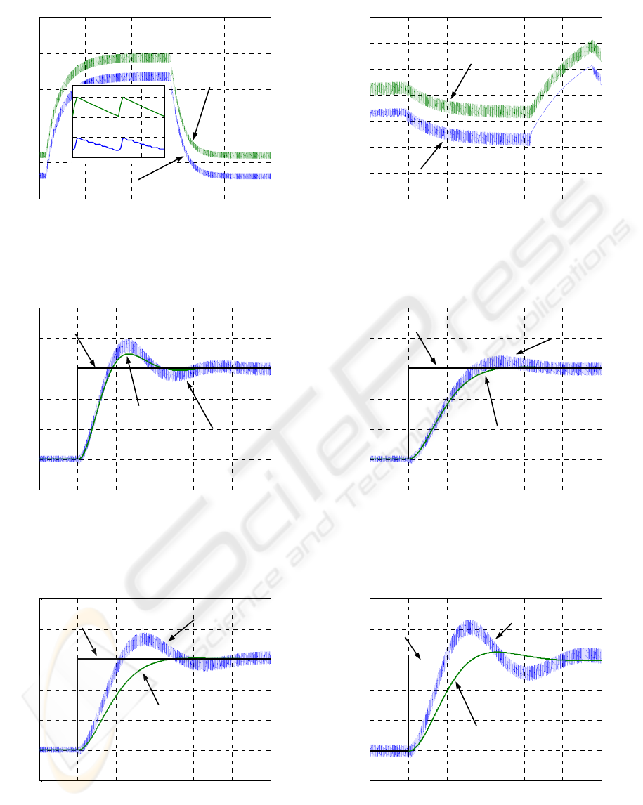
0 10 20 30 40 50
2
4
6
8
10
12
Time [s]
Pressure [bar]
Control Pressure
Rail Pressure
Figure 3: Control and rail pressures for duty cycle step
variations and constant engine speed and injectors ET
0 5 10 15 20 25 30
2
3
4
5
6
7
8
Time [s]
Pressure [bar]
Pressure Reference
Rail Pressure
(linear model)
Rail Pressure
(nonlinear model)
Figure 5: Rail pressure dynamics when the system is
controlled by a GPC with N = 5 (0.5s) and a N
U
= 1 (0.1s)
0 5 10 15 20 25 30
2
3
4
5
6
7
8
Time [s]
Pressure [bar]
PI Controller
GPC
(linear model)
Reference
Figure 7: System step responses when controlled by a PI
regulator and a GPC with N = 15 (1.5s) and N
U
= 1 (0.1s)
0 5 10 15 20 25 30
6
7
8
9
10
11
12
13
Time [s]
Pressure [bar]
Control Pressure
Rail Pressure
20.05 20.1 20.15
20
20.
2
Figure 4: Control and rail pressures for engine speed and
injectors ET step variations and constant duty cycle.
0 5 10 15 20 25 30
2
3
4
5
6
7
8
Time [s]
Pressure [bar]
Rail Pressure
(linear model)
Pressure Reference
Rail Pressure
(nonlinear model)
Figure 6: Rail pressure dynamics when the system is
controlled by a GPC with N = 15 (1.5s) and N
U
= 1 (0.1s)
0 5 10 15 20 25 30
5
6
7
8
9
10
11
Time [s]
Pressure [bar]
PI Controller
GPC
Reference
(linear model)
Figure 8: System step responses when controlled by a PI
regulator and a GPC with N = 15 (1.5s) and N
U
= 1 (0.1s),
assuming model uncertainties
A MODEL BASED CONTROL OF COMPRESSED NATURAL GAS INJECTION SYSTEMS
137