JAVA BASED TOOLBOX FOR LINEAR REPETITIVE PROCESSES
J. Gramacki §, A. Gramacki §, K. Gałkowski ‡,
∗
§Institute of Computer Engineering and Electronics, ‡Institute of Control and Computation Engineering
University of Zielona G
´
ora, ul. Podg
´
orna 50, 65-246, Poland
E. Rogers
School of Electronics and Computer Science
University of Southampton, UK
Keywords:
Repetitive processes, 2D systems, Toolbox, Java.
Abstract:
In the paper a Java based toolbox has been presented. It is used in teaching of a special case of nD systems
- Linear Repetitive Processes (LRP). Its predecessor has been developed in the Matlab environment so to use
it a Matlab licence is necessary. This restriction has been removed after making it available in the Internet
as a Java based program. Now a student, browsing a web page, may define a model together with initial /
boundary conditions, then simulate a process as a continuous or discrete case, analyze the results in graphical
or numerical form, modify visualization parameters of the plots and finally print the results. In the paper an
overview of the tool has been given.
1 INTRODUCTION
The multidimensional (Roesser, 1975), (Fornasini
and Marchesini, 1978) (nD) nature of dynamics
of Linear Repetitive Processes (Rogers and Owens,
1992) is much more difficult to understand for stu-
dents than dynamics of classical, e.g. 1-dimensional
(1D) systems. Propagation of dynamics in more than
one dimension, a built-in interactions of previous and
current system variables (called passes), causes ad-
ditional difficulties. In a repetitive process, on each
pass, an output, termed the pass profile, is produced
which acts as a forcing function on, and hence con-
tributes to the dynamics of the next pass profile. The
2D systems structure of a repetitive process arises
from information propagation in (i) the pass to pass
direction, and (ii) along a given pass. Such a process
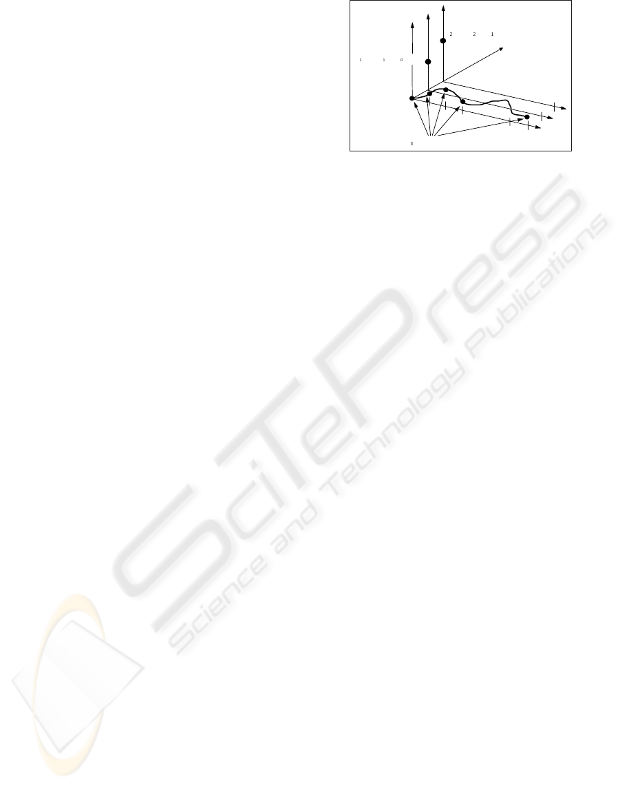
may be presented graphically – see Figure 1 below.
We quote that the explicit interaction between suc-
cessive pass profiles is the source of the novel control
(and numerical) problems for these processes in that
the output sequence of pass profiles can contain oscil-
lations that increase in amplitude in the pass to pass
direction.
Moreover, we define more than one stability no-
∗
K. Gałkowski is currently a Gerhard Mercator Guest
Professor in the University of Wuppertal, on sabbatical
leave from University of Zielona G
´
ora, {galkowsk@uni-
wuppertal.de}
tion for repetitive processes (unlike as in classical 1D
dynamic systems). A given process may be stable as-
ymptotically, stable along the pass, stable horizontally
and vertically. All of them have clear interpretation
in physical processes. This fact may potentially de-
crease students understanding of the problem.
Even ’simple’ processes (SISO case, ’smooth’ con-
trol and initial conditions, ’rounded’ matrices, etc.)
often cause ’unpredictable’ results of simulations.
Another example is that we often observe a kind of
wave oscillation that depends on the length of pass
and dynamic properties of a given process. The num-
ber of such ’anomalies’ seemed to be enough motiva-
tion to design and develop a proper educational tool.
Above we have mentioned only a few difficulties,
that we often observe during students classes. The
toolbox, in our intention, should help students in their
in-deep understanding of a fascinating nature of repet-
itive processes.
1.1 Discrete case
The state space model of a discrete linear repetitive
process has the following form (Rogers and Owens,
1992)
x
k+1
(p + 1) = A x
k+1
(p) + B u
k+1
(p) + B
0
y
k
(p)
y
k+1
(p) = C x
k+1
(p) + D u
k+1
(p) + D
0
y
k
(p)
(1)
182
Gramacki J., Gramacki A., Gałkowski K. and Rogers E. (2005).
JAVA BASED TOOLBOX FOR LINEAR REPETITIVE PROCESSES.
In Proceedings of the Second International Conference on Informatics in Control, Automation and Robotics, pages 182-187
DOI: 10.5220/0001157101820187
Copyright
c
 SciTePress

where indices k = 0, 1, . . . and p = 0, 1, . . . , α − 1
represent pass number(s) and points (position) on the
given pass respectively and
• x
k
(p) is the state vector of dimension n × 1,
• y
k
(p) is the output vector, called the pass profile
vector, of dimension m × 1,
• u
k
(p) is the bounded input vector of dimension r ×
1.
The real matrices are then as follows
A
n×n
, B
n×r
, B
n×m
0
, C
m×n
, D
m×r
, D
m×m
0
.
The constant α is a finite and fixed number called
the pass length. This model, may be clearly recog-
nized as a 2D state-space model which resembles the
well known Roesser model (Roesser, 1975). It also
posses some features of the second main 2D state-
space model, i.e. the Fornasini-Marchesini one (For-
nasini and Marchesini, 1978).
To complete the process description, it is necessary
to specify the state and pass initial conditions, i.e. the
initial state vector on each pass x
k+1
(0), k = 0, 1, . . .
and the initial pass profile y
0
(p), p = 0, 1, . . . , α − 1.
The simplest possible case is
x
k+1
(0) = d
k+1
(0), k = 0, 1, . . .
y
0
(p) = f(p), p = 0, 1, . . . , α − 1 (2)
where d
k+1
is an n × 1 vector with constant entries
and f(p) is an m × 1 vector whose entries are
known bounded functions of discrete time p. These
conditions are frequently called, by analogy to the
classical 1D systems, initial conditions. However,
in fact they are clearly boundary conditions in their
nature.
A more general form of (2) called dynamic initial
conditions (extended state initial conditions) for (1) is
defined as
x
k+1
(0) = d
k+1
(0) +
α−1
X
j=0
K
j
y
k
(j). (3)
Note. The process state space model (1) has the so–
called unit memory property, i.e. it is only the pass
profile on the previous pass which (explicitly) con-
tributes to the current one. Non–unit memory linear
repetitive processes are the natural generalization of
(1) where a finite number, say M > 1, of previous
pass profiles (explicitly) contribute to the current one.
Such processes are not considered here since the re-
sults given for the unit memory special case general-
ize in a natural manner.
1.2 Continuous case
The state space model of a differentiallinear repetitive
process has the following form over 0 ≤ t ≤ α, k =
[  G I\ M
[\
N

[  G I\ M 
\ MM a







a
a
Figure 1: Schematic illustration of the dynamics of a repet-
itive process (1) with extended version of state initial con-
ditions (3)
0, 1, . . . (Rogers and Owens, 1992)
˙x
k+1
(t) =
b
Ax
k+1
(t) +
b
Bu
k+1
(t) +
b
B
0
y
k
(t)
y
k+1
(t) =
b
Cx
k+1
(t) +
b
Du
k+1
(t) +
b
D
0
y
k
(t).
(4)
Initial or boundary conditions are defined similarly
as in the discrete case and due to space limitations we
omit them here.
To simulate (4) one must first build a discrete
equivalent of (4), hence the problem considered now
is as follows: given a repetitive process of the form
(4), construct a discrete approximation of the proper
form over p = 0, 1, . . . , α − 1, k = 0, 1, . . . i.e the
model as in (1) and (2).
The matrices in the discrete case (1) are to be com-
puted from those of (4) by formulas determined by
a particular numerical approximation method used
(Gramacki et al., 2002), (Gramacki, 2000), (Rogers
et al., 2002), (Gałkowski et al., 1999). The approxi-
mate solution generated by (1) and (2), should be as
close as possible (in a well defined sense) to the exact
solution obtained from (4) (assuming that it is known
or may be calculated with negligible errors). More-
over, crucial system properties of (4) such as stabil-
ity, should be preserved in (1) and (2) or conditions
(which can be verified numerically) under which this
is true should be given.
Figure 1 gives schematic illustration of the evolu-
tion of the dynamics of a repetitive process.
2 THE TOOLBOX
In this section we present some main features of the
toolbox (Szumacher, 2004) and describe some se-
lected technical details of its implementation.
JAVA BASED TOOLBOX FOR LINEAR REPETITIVE PROCESSES
183

2.1 Functionality
In its current state, the toolbox can, amongst other
tasks, simulate and display the response of differen-
tial and discrete linear repetitive processes and com-
pute, using a user specified numerical integration
technique, a discrete approximation to the dynamics
of a differential process. Using the toolbox in both
Java and Matlab versions we may:
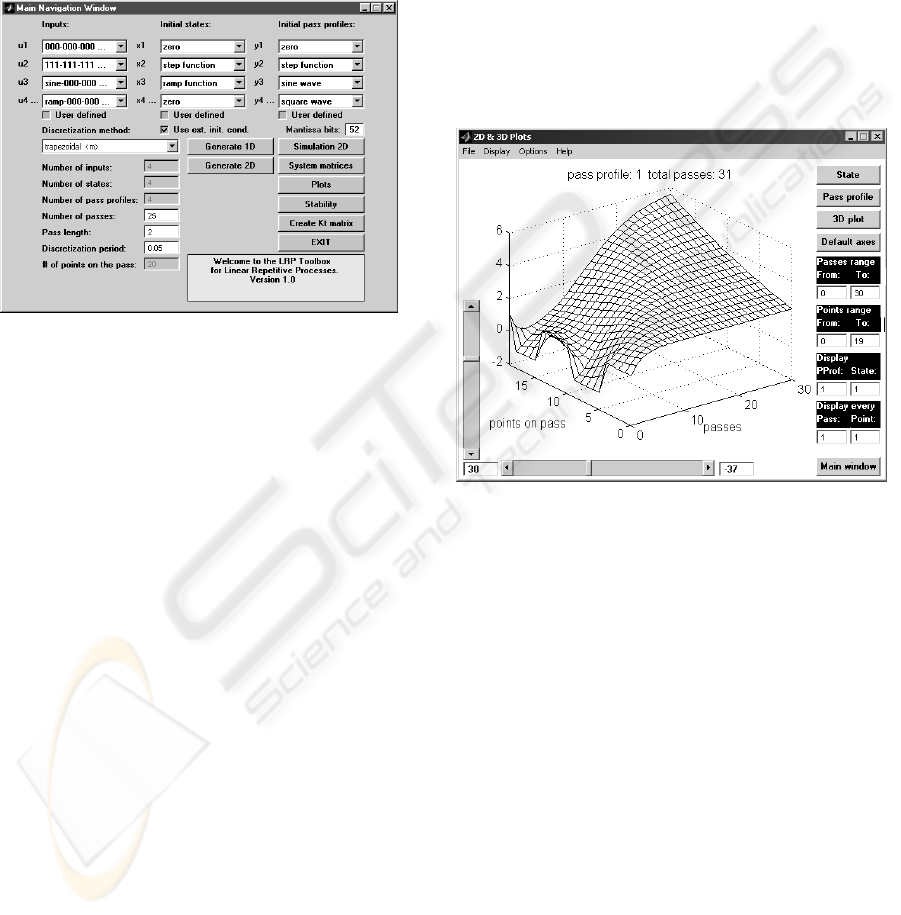
Figure 2: The Main Navigation Window of the Matlab
based version of the toolbox. A MIMO (4 inputs, 4 states,
4 outputs), continuous process (in a state ready for simula-
tion) is shown. Some elements do not appear in the Java
based version. See Table 1 for details of those differences.
• define a discrete or continuous repetitive process in
the form of system matrices in (1) or (4),
• in the case of a continuous process (4), choose a
discretization method (e.g. trapezoidal 2D approx-
imation). For a discrete case we simple choose ”no
disscretization”,
• based on process dimensions determined from sys-
tem matrices, define inputs u, initial states x
k+1
(0)
and initial pass profile(s) y
0
(p) (2) from a number
of predefined values,
• define inputs u, initial states x
k+1
(0) and initial
pass profile(s) y
0
(p) from scratch (matrix variables
of proper dimensions, taken directly from a Mat-
lab’s workspace). We may also use extended ver-
sion of state initial condition (3)(available only in a
Matlab based version),
• define ”spatial” characteristics of a process, i.e.
how many passes are to be simulated and how long
each pass is. For a discrete case, the last value is
defined as a number of points on the pass. For a
continuous case it is defined as two numbers: pass
length (in a unit of measure) and discretization pe-
riod,
• simulate a described process,
• analyze simulation results as 3D and/or 2D (Matlab
version only) plots of state(s) x and pass profile(s)
y. If necessary, one may easily narrow up and down
to a required subset of passes and a required subset
of points on a given pass,
• analyze simulation results by inspecting numerical
outputs in a dedicated Java based window or by in-
specting Matlab’s workspace variables,
• analyze stability conditions of a repetitive process
(Matlab based version only).
Figures 2 to 6 show some selected windows of both
versions of toolboxes. The Main Navigation Window
of the Java based version, due to space limitations and
its availability on the Internet has been omitted.
Figure 3: The Matlab based version. A 3D plot of results
of simulation of a given LRP process. Note the elements
which help ’visualization’ of the resulted plots (vertical and
horizontal strollers and edit boxes on the right side of the
window). The LRP process is the same as on Figure 4
2.2 Data Format Specification
Here we describe the data structures specification as
well as some other related tasks necessary to simulate
a discrete model defined by (1) and (2). The basic
user supplied data required is as follows:
• the matrices which define the LRP model,
• the pass length α,
• the number of passes, say K, over which the simu-
lation
is to be run,
• the sequence of input vectors
u
k
(p), k = {0, 1, . . . K}, 0 ≤ p ≤ α,
• the initial state vector sequence x
k
(0), k =
{0, 1, . . . K},
ICINCO 2005 - INTELLIGENT CONTROL SYSTEMS AND OPTIMIZATION
184

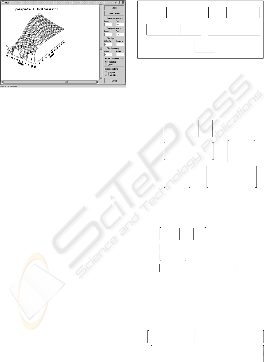
Figure 4: The Java based version. A 3D plot of results of
simulation of a given process. Note the elements which help
’visualization’ of the resulted plots (vertical and horizontal
strollers ,edit boxes and radio buttons on the right side of
the window). The LRP process is the same as on Figure 3
• the initial pass profile y
0
(p), 0 ≤ p ≤ α,
• the sampling period T .
Note: According to the convention adopted in the de-
velopment stage, the first pass is numbered 0 (zero).
Assuming this data has been supplied, the toolbox cal-
culates:
• the initial state vector for each pass
x
k
(p), k = {0, 1, . . . K}, 0 ≤ p ≤ α,
• the pass profile at each instant along each pass
y
k
(p), k = {0, 1, . . . K}, 0 ≤ p ≤ α.
Given T and α, the number of points P is calculated
according the following formula: P = (α/T ) + 1
(rounded to integer value if necessary).
Consider now the storage of the sequence of con-
trol vectors u for each pass. A natural approach would
be to store values of control sequence for a given
pass in an array of r rows (number of inputs) and
P columns (number of points). Hence there are K
passes and one should simply add a third dimension
to the array. Unfortunately, when the first release of
the toolbox appeared, MATLAB (version 4.2) did not
supported multidimensional (that is for n ≥ 3) ar-
rays. Hence the control sequences for each pass are
stored in one (potentially ’large’) two–dimensional
array where each pass occupies P respective columns.
The same method is used for the state initial state se-
quence x
0
, the initial pass profile y
0
, the computed se-
quence of state vectors x, and the computed sequence
of pass profiles y. Figure 5 gives a schematic illustra-
tion of the format of these matrices.
To illustrate the computations, consider a discrete–
time process (1) defined by the following matrices
u=
Pass 0
r × P
· · ·
Pass K
r × P
x
0
=
Pass 0
n × 1 · · ·
Pass K
n × 1
y =
Pass 0
m × P
· · ·
Pass K
m × P
x=
Pass 0
n × P
· · ·
Pass K
n × P
y
0
=
Pass 0
m × P
Figure 5: Format details of input and output vectors for lin-
ear repetitive processes (vectors u, x
0
, y
0
, x, y). r – number
of inputs, n – number of states, m – number of pass profiles
(outputs), P – number of points on a given pass, K – num-
ber of passes.
A =
1 −2 −1
3 −5 1
1 −2 0
B =
1 2
−1 −2
3 −1
B
0
=
1 1 1 1
2 2 2 2
−1 −1 −1 −1
C =
1 1 1
0 0 0
1 1 1
0 0 0
D =
1 2
1 2
−1 −2
−1 −2
D
0
=
1 1 1 1
−1 −1 −1 −1
1 1 1 1
−1 −1 −1 −1
(5)
here r = 2, n = 3, m = 4. Suppose also that α = 2,
T = 1 and hence P = (α/T ) + 1 = 3. The inputs
are as follows.
x
0
=
NaN 1 2
NaN
1 2
NaN
1 2
← x
1
0
← x
2
0
← x
3
0
y
0
=
1 1 1
1 1 1
1 1 1
1 1 1
← y
1
0
← y
2
0
← y
3
0
← y
4
0
u =
NaN N aN N aN 1 1 1 2 2 2
NaN N aN N aN
1 1 1 2 2 2
← u
1
← u
2
(6)
where the superscripts are used to denote the entries
in the corresponding vector. Here we have 3 states,
4 pass profiles and 2 inputs. Then the resulting state
and pass profile vectors for the case of K = 3 are as
follows
x =
NaN N aN N aN 1 7 16 2 7 19
NaN N aN N aN
1 2 10 2 5 4
NaN N aN N aN
1 −4 0 2 −7 12
y =
1 1 1 12 14 35 17 20 68
1 1 1
1 1 1 −1 −5 −47
1 1 1
2 4 25 7 10 58
1 1 1
−9 −9 −9 −11 −15 −57
(7)
JAVA BASED TOOLBOX FOR LINEAR REPETITIVE PROCESSES
185

where NaN (not a number) denotes entries in the
relevant matrices which are only necessary for com-
putational information purposes (the control sequence
u and initial state x
0
are not defined for pass number
0 for (4).
2.3 Implementation
The toolbox has been fully implemented in Java (Java
applets) technology and hence it can be started from
practically any WWW browser currently in use. Al-
though to use it, it is necessary to install some ’addi-
tional to standard’ software on a client machine. See
section Instalations below for details.
For a graphical user interface we used a standard
Java AWT (Abstract Window Toolkit) – the standard
API for providing graphical user interfaces (GUIs)
for Java programs (Java-AWT, 2005). For present-
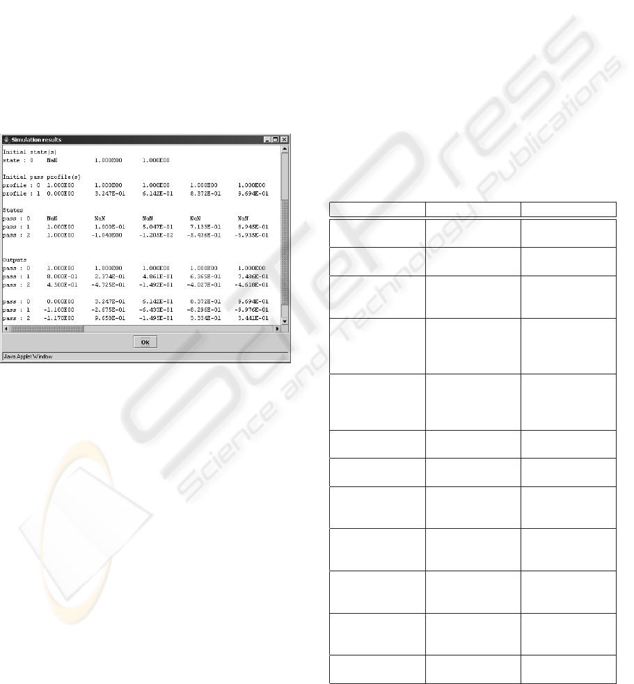
Figure 6: The Java based version. One may see, in nu-
merical format, both input data (Initial state(s), Initial pass
profile(s)) and results of simulation (States, Outputs). For
visible reasons, unnatural small number of passes = 2 was
used. A discrete MIMO process (2 inputs, 1 state, 2 outputs)
was simulated. Initial pass profiles are a square function and
a sine function.
ing graphical results of simulations we used a Java3D
library – the library for creation of three-dimensional
graphics applications and Internet-based 3D applets
(Java 3D, 2005).
For matrix operations we use JAMA package
(JAMA, 2005). JAMA is a basic linear algebra pack-
age for Java. It provides user-level classes for con-
structing and manipulating matrices. It seems that it
is intended to serve as the standard matrix class for
Java.
Due to space limitations we omit Java code exam-
ples. They are however available on request from the
authors.
In the Java based version only the basic discretiza-
tion methods for converting a continuous process to
its discrete-time equivalent have been implemented.
The following methods have been implemented: for-
ward, backward, trapezoidal, which seems to be
enough for educational purposes. See (Gramacki
et al., 2002) for more details and methods.
3 COMPARISON OF JAVA AND
MATLAB VERSIONS
Although the Java version of the toolbox seems to be
enough for student’s needs, some additional possibil-
ities are accessible only in Matlab based version. In
Table 1 we enumerate those that are important from
user’s point of view. Some limitations are due to Java
applets technology used.
Table 1: Comparison of Java and Matlab besed versions of
the toolbox
Feature Java version Matlab version
Maximum number
of simulated passes
limited unlimited
Maximum pass
length
limited unlimited
Support for ex-
tended initial
conditions (3)
no yes
Support for user de-
fined control, initial
and boundary con-
ditions
no, only predefined
values
yes, predefined val-
ues and/or any val-
ues taken from the
Matlab’s workspace
Predefined system
matrices
yes no, but user may
read them from mat-
files and/or from the
Matlab’s workspace
Stability analysis no yes, for SISO case
only
Number of dis-
cretization methods
4 14
Plot modes 3D, useful in analy-
sis of a whole
process
3D and 2D, 2D case
useful in analysis of
a single pass
Plot of a subset of
simulated points /
passes
yes yes
Calculation of a hor-
izontal and vertical
pass profiles
no yes
Results in numerical
form
yes, available
in Java applet’s
window
yes, available in the
Matlab’s workspace
Precision of calcula-
tions
fixed, 52 bits of
mantissa
variable, 1 to 52 bits
of mantissa
ICINCO 2005 - INTELLIGENT CONTROL SYSTEMS AND OPTIMIZATION
186

4 CONCLUSIONS, FUTURE
WORKS AND INSTALLATION
4.1 Conclusions
The paper shortly presents two computer tools suc-
cessfully used in teaching activities of rather complex
multidimensional systems - repetitive processes. Af-
ter an introduction of repetitive processes, the main
functionality of these tools have been given.
The two versions, based on Matlab and Java, differ
rather considerably. This was intentionally assumed.
A Java based version is intended for a wider fam-
ily of users. It is freely available from the Internet
and although shows only basic features of repetitive
processes, it seems to be enough for a starting point.
The Matlab based version is intended for a more
professional family of users. It seems to be a proper
tool in assisting of research in a field of repetitive
process and nD systems in general.
4.2 Future Works
At the moment, the Matlab based version of the tool-
box supplies much more functionality than its Java
based equivalent. It may be purposeful to enrich
somehow the last. However due to some real Java
applets limitation, not all changes will be possible
to implement. A plain Java program may also be
considered. They are also works going on to mi-
grate the Matlab based version to non-commercial
and free package for scientific and numerical compu-
tations Scilab (Scilab, 2005).
4.3 Instalation and Availability
In order to work with the applet it is necessary to in-
stall locally a Java Runtime Environment (JRE) which
allows end-users to run Java applications.
It is also necessary to install the Java3D pack-
age which enables the creation of three-dimensional
graphics and Internet-based 3D applets. One may
download it for free for Windows (Java 3D, 2005)
(first look for something like Download Java 3D x.y.z
software where x.y.z is a release number and then look
for something like Java 3D for Windows (OpenGL
Version) Runtime for the JRE). A version for Linux
is also available for free.
Due to Java applets properties / limitations, to use
for example a system clipboard sometimes it is nec-
essary to change your java.policy settings. See your
browser documentation for details. A reader may fa-
miliarize with the toolbox by visiting the page
http://www.uz.zgora.pl/˜jgramack/
LRP/lrp.html.
REFERENCES
Fornasini, E. and Marchesini, G. (1978). Doubly indexed
dynamical systems: state models and structural prop-
erties. Math. Systems Theory, (12):59–72.
Gałkowski, K., Rogers, E., Gramacki, A., Gramacki, J., and
Owens, D. (1999). Higher order discretisation meth-
ods for a class of 2-d continuous-discrete linear sys-
tems. IEE Proceedings - Circuits, Devices and Sys-
tems, 146(6):315–320.
Gramacki, A. (2000). On a new method of discretization
of differential linear repetitive processes. Bulletin of
the Polish Academy of Science: Technical Sciences,
48(4):540–560.
Gramacki, A., Gramacki, J., Gałkowski, K., Rogers, E., and
D.H., O. (2002). From continuous to discrete mod-
els of linear repetitive processes. Archives of Control
Science, 12(1–2):151–185.
Roesser, R. (1975). A discrete state space model for linear
image processing. IEEE Trans. Automatical Control,
(20):1–10.
Rogers, E., Gałkowski, K., Gramacki, A., Gramacki, J.,
and Owens, D. (2002). Stability and controllability
of a class of 2-d linear systems with dynamic bound-
ary conditions. IEEE Transactions on Circuits and
Systems - I.- Fundamental Theory and Applications,
49(2):181–195.
Rogers, E. and Owens, D. (1992). Stability Analysis for
Linear Repetitive Processes, volume 175. Springer-
Verlag.
Szumacher, D. (2004). Java toolbox for repetitive processes
(in polish). Master thesis, University of Zielona Gora,
Poland.
JAMA (2005).
JAMA: A JAva MAtrix package -
http://math.nist.gov/javanumerics/jama/.
Java 3D (2005).
http://java.sun.com/products/java-
media/3D/download.html.
Java-AWT (2005).
Java Abstract Window Toolkit
http://java.sun.com/products/jdk/awt/.
Scilab (2005).
A Free Scientific Software Package
http://scilabsoft.inria.fr/.
JAVA BASED TOOLBOX FOR LINEAR REPETITIVE PROCESSES
187