PREDICTIVE CONTROL FOR MODERN INDUSTRIAL ROBOTS
Algorithms and their applications
Květoslav Belda, Josef Böhm
Department of Adaptive Systems
Institute of Information Theory and Automation, Academy of Sciences of the Czech Republic
Pod vodárenskou věží 4, 182 08 Prague 8 – Libeň, Czech Republic
Pavel Píša
Department of Control Engineering
Faculty of Electrical Engineering, Czech Technical University in Prague
Karlovo nám. 13, 121 35 Prague 2, Czech Republic
Keywords: Predictive control, Redundant manipulators, Robotics, Steady-state error problem.
Abstract: Industrial robots comprise substantial parts of machine tools and manipulators in production lines. Their
present development stagnates in their control. Traditional approaches, e.g. NC (numerical control) systems
combined with PID/PSD structures, provide control of the tool drives as separate units only, but not solve
the control from view of the whole machine system. On the other hand, in control theory, there are a lot of
approaches, in which the information on tool dynamics and kinematic relations can be involved. The main
contribution of this paper is to introduce various utilization and modifications (not only control tasks) of one
such approach – model-base predictive control. The control is being developed for modern industrial robots
based on parallel configurations. The modifications of predictive algorithm are substantiated by real
laboratory experiments. The paper concerns with basic control design and its possibilities to remove
positional steady-state error. Quadraticaly-optimal trajectory planning is outlined in it.
1 INTRODUCTION
Industrial robots comprise substantial parts of ma-
chine tools and manipulators in production lines.
Their present development stagnates in their control,
which should ensure not only high accuracy, but also
economical and safe operation.
Traditional approaches, e.g. Numerical Control
systems (NC
systems) combined with PID/PSD stru-
ctures, provide control of the robots only from view
of their drives considered as separate units. It means
that whole robotic system is taken into account
as a set of drives and their relations. These relations
are given by mechanical constrains arising from real
robot structure – real mechanism. In those appro-
aches, the relations are considered only as distur-
bances acting to individual drives. This concept
yields no possibilities for further increase of opera-
tional accuracy and load capacity.
Modern control approaches can involve the most
of properties of whole robotic system through its
mathematical model. It is obtained by virtue of ma-
thematical-physical analysis or some numerical
identification method. Such control approaches are
generally called model-based approaches. They can
design, just by use of the mathematical model,
corresponding and energetically reasonable control
actions.
One of modern model-based approaches is multi-
step Predictive control (Ordys and Clarke 1993). It is
applicable in new developed industrial robots (e.g.
Neugebauer, ed., 2002), which are based on redun-
dantly actuated parallel structures. They represent
multi-input multi-output systems and their redundant
actuation solving the problem of workspace
singularities (Belda et al. 2003) deter mines different
number of their inputs and outputs.
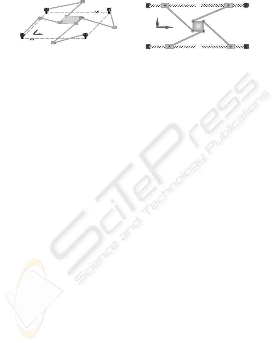
In use of parallel robots, model-based control
can be fully utilized, for more complicacy of the
robot structure. Control based on model can better
distribute the input energy in the structure. Example
of two parallel structures is shown in Figure 1.
3
Belda K., Böhm J. and Píša P. (2005).
PREDICTIVE CONTROL FOR MODERN INDUSTRIAL ROBOTS - Algorithms and their applications.
In Proceedings of the Second International Conference on Informatics in Control, Automation and Robotics - Robotics and Automation, pages 3-10
DOI: 10.5220/0001155800030010
Copyright
c
 SciTePress

drive3
y
x
drive1 drive2
drive4 drive3
y
x
drive1 drive2
drive4
drive1
drive4
z
drive3
x
drive2
drive1
drive4
z
drive3
x
drive2
‘Crosshead’ ‘Sliding Star’
Figure 1: Planar parallel robots: horizontal and vertical
Although the parallelism is appeared in robotics
in the sixties - Stewart platform in 1965 (Tsai,
1999), their wider development started in the nine-
ties (Neugebauer, ed., 2002). The parallel robots are
promising way, how to significantly improve accu-
racy, speed and stiffness of machine tools. They can
be simply understood as movable truss constructions
or as movable work platforms supported by a set
of parallel arms (Tsai, 1999).
The main contribution of this paper is to demon-
strate various utilization and modifications (not only
control tasks) of predictive control; if it can achieve
acceptable dynamic control errors and solve steady-
state error problem. The theoretical results imple-
mented in algorithms are substantiated by real
laboratory experiments with redundant parallel
structure ‘Sliding Star’ (Figure 1, 3).
2 MODEL-BASED APPROACH
The model-based approaches use the model as prior
information (feed-forward). It enables to predict
future behavior of a controlled system. Considering
future requirements and behavior, the input energy
can be optimized (Ordys and Clarke, 1993).
The models can be expressed in different forms.
In case of multi-input multi-output structures
(MIMO systems), as robots are, the model is useful
expressed by state-space formulation. State-space
model more clearly expresses the relations among
inputs and outputs and their coupling.
2.1 Composition of the Robot Model
Generally, the robot is a multibody system. Its
model is represented by pure equations of motion.
They are composed mostly from Lagrange’s
equations (e.g. Stejskal and Valášek, 1996). Then
the mathematical model described the real system
is given by a set of differential equations (1)
uyyyy )(),( gf +=

(1)
where input vector u can represent only forces,
caused by torques on drives in case of horizontal
configuration
τ
Fu
=
(2)
or these forces enlarged by gravitational forces
in case of vertical configuration
τ
FFu +−=
g
(3)
The equations (2) and (3) serve for final
determination of real control actions – force effects
required from drives. Furthermore, this arrangement
provides the equality
0yy =),(

f for arbitrary y from
range of definition and zero time derivatives
0y
=

in spite of presence of gravitational forces, which are
added to inputs (equation (3)).
The function
),( yy

f produces that the equation
(1) is nonlinear for state
TT
],[],[
21
xxyyX ==

.
One of ways to cope with nonlinearity is to use some
kind of linearization. In the following subsection,
one linearizing technique is introduced.
2.2 Exact Linearization
The subsection 2.2 deals with the linearization based
on differences. Against standard linearization using
partial derivatives, the resultant form is usable not
only in the working point, but also in its wider
neighbourhood.
The nonlinearity in the equation (1) can be
linearized as follows (Valášek and Steinbauer, 1999)
yyyyyyyy

),(),(),(
21
aa +=f
(4)
and transformed in state-space form
⎥
⎦
⎤
⎢
⎣
⎡
⎥
⎦
⎤
⎢
⎣
⎡
=
⎥
⎦
⎤
⎢
⎣
⎡
=
2
1
21
),(
)(
x
x
aa
10
yy
y
Xf


f
(5)
Provided that the nonlinear function
),( yy

f
and point
TT
],[],[
21
xxyyX ==

are given; X
belongs to the range of definition of the function;
zero elements in X are substituted by suitable
nonzero number
0→
κ
to prevent zero division.
Furthermore, two types of state variables are
assumed: generally outputs x
1
= y and their time
derivatives x
2
= y

; i.e.
TTT
xxxx ]],,[],,,[[],[],[
2221121121
""

=== xxyyX
(6)
ICINCO 2005 - ROBOTICS AND AUTOMATION
4

Finally, the assumption from previous section
has to be also fulfilled for arbitrary y and zero
y

]
2
arbitrary,
1
[)(),( 0xxXX0Xfyy =====
rrr

f
(7)
Then the decomposition indicated by equation
(4) can be reached. Its algorithm starts from second
state variables x
2
(i.e. according to the equation (6):
order is
{x
21
, x
22
, ···, x
11
, x
12
, ···} i.e. {21, 22, ···, 11, 12, ···}) (8)
The order is given by amount of the information
included in the function f(X) and assumption (7).
The indicated order of selection will considerably
simplify decomposition, as it will be shown later.
In view of previous assumptions, the exact
linearization-decomposition is expressed as follows:
++∆
∆
∆
+∆
∆
∆
= "
DD
12
12
11
11
.
)(
.
)(
)( x
x
x
x
ff
Xf
"
DD
+−
−
∆
+−
−
∆
+ )0(
)0.(
)(
)0(
)0.(
)(
22
22
21
21
x
x
x
x
ff
(9)
(Note: The dots before variables in denominators
mark division ‘element by element’; division of all
elements of differences by scalar ∆
xij .)
In detail, the equation (9) is written that way
=)(Xf
···
.
)]([)]([
···)(
).(
)]([)]([
21
21
23
,
22
,0,
13
,
12
,
1123
,
22
,
21
,
13
,
12
,
11
1111
1111
0,0,0,
13
,
12
,
11
0,0,0,
13
,
12
,
11
+
−
+
+−
−
−
=
x
x
xx
xx
T
xxxxx
T
xxxxxx
r
r
T
xx
r
x
T
xxx
ff
ff
(10)
The individual fractions of the equation (10) are
columns of the coefficients of the matrices
),( yya

1
and
),(
2
yya

with following internal structures
0yya =),(
1

,
⎥
⎥
⎥
⎦
⎤
⎢
⎢
⎢
⎣
⎡
=
%#
"
22
2
21
2
12
2
11
2
2
aa
aa
a
(11)
The first column group (matrix
),(
1
yya

)
contains only zeros due to differences being also
zeros - the vector function equals zeros for zero time
derivatives; see equation (6) – e.g. numerator of the
first column of
),(
1
yya

is
0ff =− )]0,0,0,,,([)]0,0,0,,,([
131211131211
T
r
T
xxxxxx
(12)
2.3 Discrete State-Space Formulation
Let the linear (or linearized) differential equation
or the system of differential equations with separate
the highest derivation on left side are assumed
uyyyyyyyyyfy )(),(),(),( g++==

21
aa
(13)
Then, its continuous state-space form is written as
⎥
⎥
⎥
⎦
⎤
⎢
⎢
⎢
⎣
⎡
=
⎥
⎥
⎥
⎦
⎤
⎢
⎢
⎢
⎣
⎡
=
⎥
⎥
⎥
⎥
⎦
⎤
⎢
⎢
⎢
⎢
⎣
⎡
=
+=
)(
;;
1
21
2
1
x
0
B
aa
10
A
x
x
X
uBXAX
g
CC
CC

[]
21
ccC
XCy
=
=
C
C
(14)
For real-time control the system (14) has to be
discretized, because continuous realization is not
feasible. The reason is that the model of the robot
needs certain time for its own composition and real
control systems are usually realized discretely.
The discretization of the model has to be realized
also in finite time. Therefore, the conventional
discretization technique (Šulc, 1999)
)()()1(
)(
kdekek
k
k
C
k
CC
uBXX
AA
∫
+
−+
+=+
δδ
δ
τδδδ
τ
(15)
is provided by finite expansion of exponential
function
)( ⋅
e .
Finally, then the discrete state-space model is
written as follows
)(
)(
)(
)(
)1( k
k
k
k
k uB
X
X
C
A
y
X +
=
=+
(16)
This model (16) is initial form for further
explanation of design of predictive algorithm.
3 PREDICTIVE CONTROL
Generalized Predictive Control is a multi-step con-
trol (Ordys and Clarke, 1993) as well as a similar
approach – Linear Quadratic Control (Phillips and
Nagle, 1995). It offers more powerful control actions
than standard PID controllers and therefore it gains
significant and widespread application in industrial
process control. Its basic formulation can be
adapted, without difficult modifications, for multi-
input multi-output (MIMO) systems.
The control is based on local optimization
of quadratic cost function (quadratic criterion)
()()
{}
+−−=
∑
+=
++++
N
Noj
jkjk
T
jkjk
k
J
1
)()()()(
wyQwy
y
{}
∑
=
−+−+
+
Nu
j
jk
T
jk
1
)1()1(
uQu
u
(17)
The criterion is expressed in step k. N is a hori-
zon of optimization, No is a horizon of initial
insensitivity and Nu is a control horizon.
Q
y
and Q
u
are output and input penalizations and
y
(k+j)
and
u
(k+j −1)
are input and output values.
PREDICTIVE CONTROL FOR MODERN INDUSTRIAL ROBOTS - Algorithms and their applications
5

The predictive control combines together both
feed-forward part and feed-back part. The former,
feed-forward part is represented by prediction
via mathematical model of the controlled system
(parallel robot). It forms the dominant part of control
actions. The latter, feed-back, closed from measured
outputs, compensates some model inaccuracies
and certain bounded disturbances.
In spite of mentioned incontestable advantages of
predictive control, it can cause, in general point
of view, occurrence of steady-state errors. It is
happened not only when penalizations in quadratic
cost function are nonzero but also e.g. when
unmeasured disturbances occur.
It can be solved by modification of generalized
predictive algorithm, which will be explained
thereinafter.
3.1 Equations of Prediction
The prediction is fundamental part of the design.
It defines the character of the algorithm. Generally,
let us consider two types of algorithms:
• absolute algorithm (standard)
• incremental algorithm (modified standard)
Absolute algorithm generates directly values
of the control actions, their full (absolute) values.
The algorithm arises from the model (14) or (16)
without any changes. On the other hand, incremental
algorithm generates only increments of the control
actions. To obtain incremental/integrative character,
the integrator has to be added to the model of the system.
The following lines show this addition
uyyyyyyyyyfy )(),(),(),( g++==

21
aa (18)
uduuduu
~
)(' ==→=
∫
tdt (19)
after insertion of equation (19) to (18), it is obtained
uyyyyfy
~
'''))',((''' g++==
21
aa

(20)
Then continuous state-space formulation is
u
0
0
x
x
x
10
0
0
010
x
x
x
~
][][
3
2
1
21
3
2
1
⎥
⎥
⎦
⎤
⎢
⎢
⎣
⎡
⎥
⎦
⎤
⎢
⎣
⎡
+
⎥
⎥
⎥
⎦
⎤
⎢
⎢
⎢
⎣
⎡
⎥
⎥
⎥
⎦
⎤
⎢
⎢
⎢
⎣
⎡
⎥
⎦
⎤
⎢
⎣
⎡
⎥
⎦
⎤
⎢
⎣
⎡
=
⎥
⎥
⎥
⎦
⎤
⎢
⎢
⎢
⎣
⎡
g
aa



(21)
⎥
⎦
⎤
⎢
⎣
⎡
⎥
⎦
⎤
⎢
⎣
⎡
⎥
⎦
⎤
⎢
⎣
⎡
+=
===
C
C
C
C
CC
B
0
B
A0
010
AX
x
x
x
uBXAX
~
;
][
~
;
~
3
2
1
~
~~
~
~

TT
ccC ]'',',[],,[];[
~
321
~
~
yyyxxxX0CCXCy ====
(22)
Extended state
X
~
is computed by state observer
(Anderson and Moore, 1979). This modified model
(22) has the same form as state-space model (14).
If it is discretized according to (15), then obtained
model is the same as (16). That form is generally
correct and it will be used in the following text also
for the modification (21) and (22).
Using considered discrete state-space form (16),
the equations of prediction are usually expressed as
)1(
)1(
)(
)(
)(
)(
1
1
)(
)(
)(
)(
)(
)(
)1(
)1(
−+
−+
−
−
+
+
+
+
+
+
+
+
+
+
+
+
=
=
=
=
Nk
Nk
k
k
k
k
N
N
k
k
k
k
N
N
Nk
Nk
k
k
Bu
Bu
CBu
Bu
Bu
Bu
A
A
C
C
X
X
X
X
A
A
A
A
C
C
y
X
y
X
"
"
%##
#




(23)
and in matrix notation, they are given that way
uGfy +=

() k
N
X
CA
AC
f
⎥
⎥
⎥
⎦
⎤
⎢
⎢
⎢
⎣
⎡
= #
,
⎥
⎥
⎥
⎦
⎤
⎢
⎢
⎢
⎣
⎡
=
−
CB
0
B
B
AC
C
G #
"
%
"
#
1N
(24)
Vector
f represents free responds (u = 0) from time
instant k. The product
G u compensates differences
of free responds from desired values within horizon
of optimization N (Ordys and Clarke, 1993).
3.2 Computation of Control Actions
The control actions are obtained by minimization
of quadratic criterion (17). It can be simply rewritten
to the following matrix product (Belda et al. 2002)
=
⎥
⎦
⎤
⎢
⎣
⎡
−
⎥
⎦
⎤
⎢
⎣
⎡
⎥
⎦
⎤
⎢
⎣
⎡
−
=
u
wy
Q0
0Q
Q0
0Q
uwy
u
y
u
y


],)[(
TT
k
J
JJ ×=
T
(25)
where y

is a vector composed according to (24)
(time step k+1, · · ·, k+N), w is a vector of desired
values, corresponding to vector
y

and u is a vector
of designed future inputs, again in discrete time
instants for the whole horizon (k, · · ·, N - 1).
The product (25) is more suitable form that can
be decomposed in two parts so-called square roots
of the criterion. From mathematical point of view
the minimization of square root is more straight-
forward.
If the square root of the criterion on the right side
is selected and expression of prediction (24)
is inserted in this square root, then the criterion is
given
⎥
⎦
⎤
⎢
⎣
⎡
−
−
⎥
⎦
⎤
⎢
⎣
⎡
=
⎥
⎦
⎤
⎢
⎣
⎡
−
⎥
⎦
⎤
⎢
⎣
⎡
=
0
fwQ
u
Q
GQ
u
wy
Q0
0Q
J
y
u
y
u
y )(

(26)
J is a column vector and its Euclidean norm equals
a cost of the square root of the criterion.
ICINCO 2005 - ROBOTICS AND AUTOMATION
6

The objective is to search for such u, which
minimizes the square root (26) i.e. the control u
minimizes the norm |J| of the criterion. In case of
square root (26), the minimization leads to a system
of algebraic equations with more rows than
columns – over-determined system:
0
0
fwQ
u
Q
GQ
y
u
y
=
⎥
⎦
⎤
⎢
⎣
⎡
−
−
⎥
⎦
⎤
⎢
⎣
⎡
)(
0buA =−
(27)
For optimization of the criterion, the orthogonal
triangular decomposition (Golub and Van, 1989;
Lawson and Hanson, 1974) is used. It reduces
excess rows of matrix A [(2·N·i)×(N·i)] and elements
of vector b [2·N·i] (i is a number of DOF) into upper
triangular matrix R and a vector c according
to the following scheme:
T
TT
Q
b
b
Qu
u
A
A
Q
/
=
=
cuR =
(28)
⇒
=
A u
b
=
R
1
0
u c
c
z
1
(29)
Vector c
z
is a lost vector, whose Euclidean norm
|c
z
| is equal value of square root √J (i.e. J = c
z
T
c
z
).
To obtain unknown control actions u, only upper
part of the system (29) is need
11
1
1
)( cR
c
u
uR
T
=
=
(30)
Since a matrix R
1
is upper triangle, then the con-
trol u is given directly by back-run procedure.
The penalizations Qu and Qy (usually selected
as
Qy = diag(λ
y
), λ
y
=1 and Qu = diag(λ
u
), 〉〈∈ 1,0
u
λ )
determines magnitude of the redistributed loss
in considered horizon of the prediction N.
The horizons Nu and No have not direct
utilization here. Control horizon Nu is usually equal
horizon of prediction N; lower values provide
equality of control actions at the end of optimization
horizon – useless for robot motion. Initial insen-
sitivity horizon No is also directly useless. It causes,
that control differences at the beginning of the hori-
zon N are not considered.
The different choice of ratio of penalization λ
u
/λ
y
together with horizon N enables to generate control
actions that the available drives were not fitfully
exerted. However, distributed changes of torques
are achieved with the cost of certain loss (error),
that theoretically equals value of the criterion.
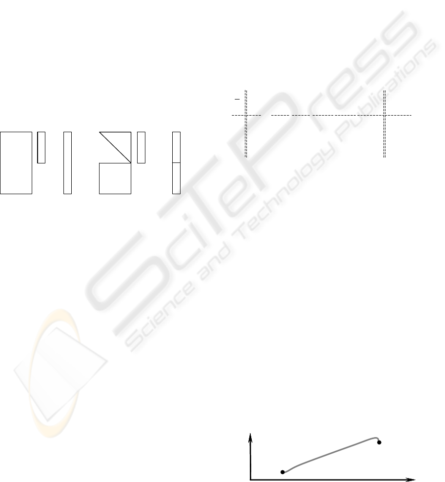
3.3 Quadraticaly-Optimal Trajectories
As one interesting possibility, the predictive control
offers, due to its several horizons (N, No, Nu), planning
trajectories by record of outputs from simulation.
The task is defined as follows: let us have two points
– start and end, and at the same time, a path
(trajectory) is not conditioned, only end-point must
be achieved (Figure 2). In such case, we can use
predictive control with specific setting of the output
horizons N and No. If we set, that the horizon
maxNN
=
and kNNo
−
=
, where k is order of the
controlled system, then the quadratic criterion will
consider only last k differences among predicted
end-point and its reference value. Thus, the matrix G
and corresponding differences (w - f) in the criterion
(27), are reduced only on their last k rows and
elements respectively
⎥
⎥
⎥
⎥
⎥
⎥
⎥
⎥
⎥
⎥
⎥
⎦
⎤
⎢
⎢
⎢
⎢
⎢
⎢
⎢
⎢
⎢
⎢
⎢
⎣
⎡
−
−
=
⎥
⎥
⎥
⎥
⎥
⎥
⎥
⎥
⎥
⎥
⎥
⎦
⎤
⎢
⎢
⎢
⎢
⎢
⎢
⎢
⎢
⎢
⎢
⎢
⎣
⎡
−
⋅
⋅
−
−−
−
0
0
fw
fw
1
0
CB
0
.
CAB
.
.
.
1
CB
.
BCA
0
1
BCA
BCA
0
0
fw
10
1
01
G
#
#
#
#
"
"
"
"
"
"
"
#
#
#
N
kN
NN
kN
)(
)(
21
(31)
Lower unit matrix in (31) corresponds to dimen-
sion of input penalization. Such form, specifically
last k rows of matrix G and corresponding
differences (w – f), causes quadratic distribution
of energy to individual inputs (control actions)
within whole horizon Nmax.
If indicated procedure would be applied, then the
control process has no information, in which step
should stop. Difference of horizons N and No is still
the same. Information on stopping the control
process is given by horizon No.
Described sequence represents specific dead-
bead control spread within time. Thus, it is not
necessary to achieve end point during minimal
number of steps (= order of system) in control
process, but on the other hand (from reasons of
feasibility by drives) it is better to distribute the
input energy uniformly without rapid turns in some
wider horizon. Its length should arise from
technological requirements.
The sequence can be used only once under
condition, that the system is linear and horizon No is
a little bit lower than horizon N; i.e. value No gives
the length of horizon, on which the system should
stop after previous
)( No-maxN steps.
Figure 2: One example of planned trajectory
z
xx
end
star
t
PREDICTIVE CONTROL FOR MODERN INDUSTRIAL ROBOTS - Algorithms and their applications
7

In case of nonlinear systems, the sequence has
to be repeated with progressively shortened horizon N
min,minmax max, NN,-NNN 1,1: += "
(32)
where the value
minN is suitable selected,
not exceed number approx. 20 (k < Nmin < 20).
The higher numbers do not improve the process.
The repetition provides the changes of model during
planning of the trajectory according to real state
of the controlled system i.e. it respects nonlinearity
by changing of models in compliance with real
positions and velocities of the robot.
4 LABORATORY EXPERIMENTS
RESULTS AND CONCLUSIONS
For laboratory tests, robot ‘Sliding Star’ was used.
It represents vertical planar parallel configuration
with different levels of potential energies (i.e. gra-
vitational force has to be considered) and redundant
actuation. The aim of the experiments was control
based on described predictive algorithms (control
circuit in Figure 4) fulfilling a given trajectory (time
histories of control process Figure 5 and 6).
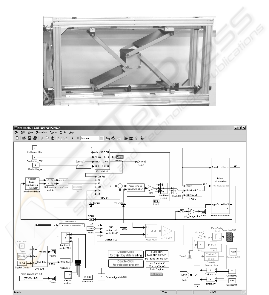
Figure 3: Lab model of parallel robot ‘Sliding Star’
Figure 4: Control scheme for predictive control and PSD controller for comparison (discrete form of PID)
ICINCO 2005 - ROBOTICS AND AUTOMATION
8

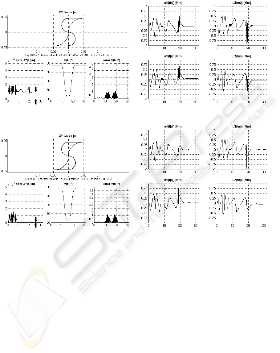
Figure 5: Absolute GPC – Steady state error is evident (ts = 0.02s; N = 10, Nu = 10, No = 0, λ
u
= 1e-6)
Figure 6: Incremental GPC – Steady state error converges to zero (ts = 0.02s; N = 10, Nu = 9, No = 1, ∆ λ
u
= 1e-6)
The control circuit (Figure 4) is composed
in MATLAB-Simulink environment, where the pre-
dictive control algorithm itself was realized as cap-
sulized C-coded s-function in Simulink block (Belda
et al. 2004). This control circuit (Simulink scheme),
after its compilation and uploading to digital signal
processor, was used for real time tests of control
on laboratory model of parallel robot ‘Sliding Star’
(Figure 3). The robot model has three degrees
of freedom (movement in direction x and z and
rotation
ψ around perpendicular axis y), but it is
redundantly actuated by fourth rotational DC motors
with gearings and motion screws. The screws
provide transformation of rotation of the motors
to straight-line motion.
The circuit contains not only the block of con-
troller and block representing robot interface, but
also other necessary blocks as blocks of generating
trajectory, model composition, discretization, kine-
matical transformations, measurement of current,
safety logical blocks etc.
The Figures 5 and 6 well present the difference
of the results of real control process with different
predictive algorithms.
In the upper parts of figure left sides, the testing
trajectory (shape ,S’) is shown. In lower parts, there
are consecutively time histories of position error,
desired rotation (besides rectilinear motion the robot
performs also rotation), and just error of rotation.
On right sides of the figures, there are times
histories of foursomes control actions – real values
of torques on appropriate drives.
The Figure 6 shows the improvement of control
process, when the incremental modification of pre-
dictive algorithm is used. Indicated error in position
in steady-state (let us say undesirable offset) is
evident in Figure 5. On the other hand, the error
in Figure 6 converges to zero.
error
error
PREDICTIVE CONTROL FOR MODERN INDUSTRIAL ROBOTS - Algorithms and their applications
9

0 1 2 3 4
-0.2
-0.1
0
0.1
0.2
time [s]
ex = xd-x [m]
0 1 2 3 4
-0.2
-0.1
0
0.1
0.2
time [s]
ey = yd-y [m]
01234
0
0.1
0.2
time [s]
exy = sqrt(e
2
)[m]
0 1 2 3 4
-20
-10
0
10
20
time [s]
error = psid-psi [°]
0 1 2 3 4
-0.2
-0.1
0
0.1
0.2
time [s]
ex = xd-x [m]
0 1 2 3 4
-0.2
-0.1
0
0.1
0.2
time [s]
ey = yd-y [m]
01234
0
0.1
0.2
time [s]
exy = sqrt(e
2
)[m]
0 1 2 3 4
-20
-10
0
10
20
time [s]
error = psid-psi [°]
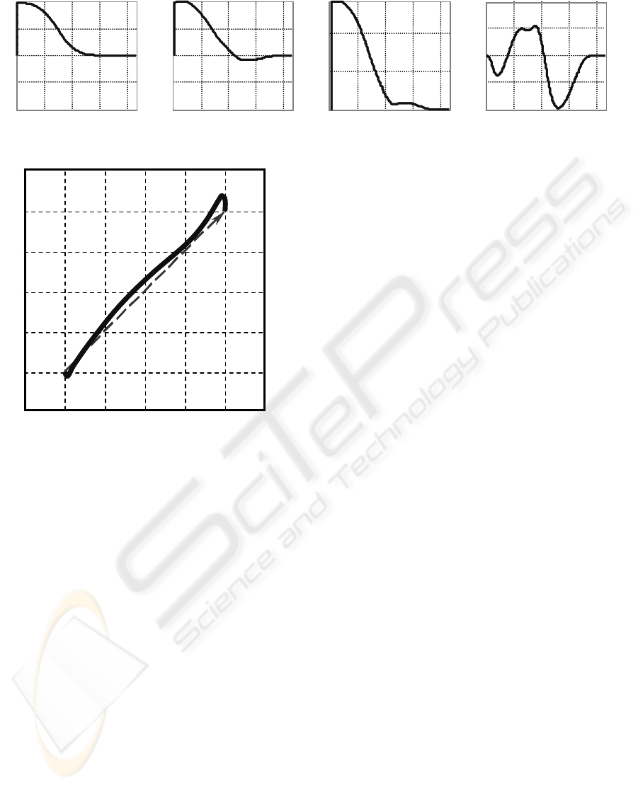
Figure 7: Time histories of differences at quadratically-optimal trajectory planning for trajectory in Figure 8
-0.1 -0.05 0 0.05 0.1
-0.1
-0.05
0
0.05
0.1
-0.1 -0.05 0 0.05 0.1
-0.1
-0.05
0
0.05
0.1
Figure 8: Really planned trajectory for ‘Sliding Star’
On the basis of shown results (representative
selection only) model-based control can be effective.
It can achieve acceptable control errors. Model-based
control can also meet some additional requirements
not only from control point of view. One of examples
can be quadratically-optimal trajectory planning (exam-
ple in Figures 7 and 8) described in subsection 3.2.
The presented simple trajectory planning is basic
idea, which can solve avoidance of obstacles not
only in robot workspace.
ACKNOWLEDGEMENTS
The authors appreciate the kind support by the Grant
Agency of the Czech Republic:
●
grant (101/03/0602, 2003/05), “Redundant drives
and measurement for hybrid machine tools”
and
●
grant (102/05/0271, 2005/07), “Methods of Predic-
tive Control, Algorithms and Implementation”.
REFERENCES
Anderson, B.D.O. and Moore, J. B. (1979). Optimal
Filtering, Prentice-Hall, Inc.
Belda, K., 2002. Control of Redundant Parallel Structures
of Robotic Systems, Dissertation, Czech Technical
University in Prague.
Belda, K., Böhm, J., and Valášek, M., 2003. State-Space
Generalized Predictive Control for Redundant Parallel
Robots. Mechanics Based Design of Structures and Ma-
chines, Marcel Dekker, Vol. 31, No. 3, pp. 413 - 432.
Belda, K., Böhm, J., Píša, P., Valášek, M. (kbweb © 2004)
GPC pages: http://www.utia.cas.cz/AS/belda/.
Golub, H., G. and Van, Ch., F., L., 1989. Matrix Compu-
tations, The Johns Hopkins Univ. Press.
Lawson, Ch. and Hanson, R., 1974. Solving Least Square
Problems, Prentice-Hall, Inc., New York.
Neugebauer, R.
ed., 2002. Development Methods and Application
Experience of Parallel Kinematics, Reports from the IWU
Vol. 16, ISBN 3-928921-76-2, IWU Chemnitz.
Ordys, A. and Clarke, D., 1993, A State - Space Des-
cription for GPC Controllers. Int. J. Systems SCI.,
Vol. 24, No. 9, pp. 1727 - 1744.
Phillips, L., and Nagle, T., 1995. Digital Control Systems
Analysis and Design, Prentice Hall, New Jersey.
Sciavicco, L. and Siciliano, B., 1996. Modeling and
Control of Robot Manipulators, The Mc-Graw Hill
Companies, Inc., New York.
Stejskal, V. and Valášek, M. 1996. Kinematics and Dyna-
mics of Machinery, Marcel Dekker, New York.
Šulc, B., 1999. Theory of automatic control. Script
of the Czech Technical University, Prague (in Czech).
Tsai, L.-W., 1999. Robot analysis, The Mechanics of Se-
rial and Parallel Manipulators, John Wiley & sons,
Inc., New York.
Valášek, M. and Steinbauer, P., 1999. Nonlinear Control
of Multibody Systems, Euromech, pp. 437-444, Lisabon.
ICINCO 2005 - ROBOTICS AND AUTOMATION
10