An Innovative Obstacle Avoidance Algorithm for UAV Based on
Hemispherical Optimal Path
Jiandong Guo
1
a
, Zhenquan Qian
2
b
, Mengjie Zhu
3
c
, Hui Liu
4
d
and Zhenguang Liu
2
e
1
Key Laboratory of Unmanned Aerial Vehicle Technology of the Ministry of Industry and Information Technology, Nanjing
University of Aeronautics and Astronautics, Nanjing, P. R. China
2
College of Automation Engineering, Nanjing University of Aeronautics and Astronautics, Nanjing, P. R. China
3
Shanghai Electro-Mechanical Engineering Institute, Shanghai, P. R. China
4
College of Aerospace Engineering, Nanjing University of Aeronautics and Astronautics, Nanjing, P. R. China
Keywords: Obstacle Avoidance Algorithm, Path Planning, Nonlinear Guidance Law, Hemispherical Optimal Path, 3D
Trajectory Tracking.
Abstract: A novel three-dimensional (3D) autonomous real-time obstacle avoidance algorithm based on hemispherical
optimal path is proposed in this paper to solve the problem of obstacle avoidance during the flight for UAVs.
Firstly, the irregular obstacles are modelled by one or more hemispheres, which are used to cover the whole
or key parts of the obstacles. Then, the avoidance strategy is obtained and the optimal arc avoidance trajectory
is calculated according to the geometric relationship between the obstacle model and UAV, and the obstacle
avoidance problem is transformed into the avoidance trajectory tracking problem. Finally, according to the
fixed distance limit of the nonlinear guidance parameters, the variable gain virtual reference point is designed,
the stability condition of trajectory tracking is analyzed, and combined with altitude guidance law to develop
the 3D trajectory tracking control and autonomous real-time obstacle avoidance. The nonlinear numerical
simulation of a type of UAV shows that the presented obstacle avoidance algorithm can avoid obstacles
effectively with high accuracy for 3D trajectory tracking, which can be applied to UAV’s obstacle avoidance
missions.
1 INTRODUCTION
Unmanned aerial vehicles (UAV) have been widely
used in civil and military fields due to their
advantages of flexibility, portability, mobility, and
concealment (Mairaj et al., 2019; Hildmann and
Kovacs, 2019). However, the flight environment will
become more and more complex with the continuous
development of UAV, the autonomous obstacle
avoidance technology of UAV will gradually become
one of the key technologies (Lacono and Sgorbissa,
2018; Wan et al., 2019).
The obstacle avoidance methods for UAV can be
mainly divided into the following two categories: (1)
a
https://orcid.org/0000-0002-4733-2550
b
https://orcid.org/0000-0003-0361-8546
c
https://orcid.org/0000-0003-2643-490X
d
https://orcid.org/0000-0003-0253-9651
e
https://orcid.org/0000-0002-8121-2990
The first method is based on path planning, the main
idea of this method is to convert the obstacle
avoidance problem to path planning problem. With
the development of research in this field, many path
planning approaches have been proposed, such as
genetic algorithm (GA) (Elhoseny et al., 2018;
Kwasniewski and Gosiewski, 2018), artificial
potential field (APF) (Tang et al., 2019; Zhang et al.,
2018), A* algorithm (Gochev et al., 2017), RRT (Zu
et al., 2018), etc., these algorithms are compared in
terms of time of computation and optimality of
solution in different scenarios and obstacle
layouts(Radmanesh et al., 2018; Zammit and Erik-
Jan, 2018), which find that the GA shows less
Guo, J., Qian, Z., Zhu, M., Liu, H. and Liu, Z.
An Innovative Obstacle Avoidance Algorithm for UAV Based on Hemispherical Optimal Path.
DOI: 10.5220/0012243300003612
In Proceedings of the 3rd International Symposium on Automation, Information and Computing (ISAIC 2022), pages 835-844
ISBN: 978-989-758-622-4; ISSN: 2975-9463
Copyright
c
 2023 by SCITEPRESS – Science and Technology Publications, Lda. Under CC license (CC BY-NC-ND 4.0)
835

sensitivity to time with respect to the increase number
of cells; the APF shows a reasonable time of solution,
but poor ability to overcome the local minima and
provides non-optimal results; the A* algorithm shows
the ability to solve the scenarios optimally by
spending considerably higher computational time, the
RRT algorithm shows faster converges, but is often
not optimal. In general, there is a trade-off between
the optimality and computational time requirements
in path planning algorithms (Agarwal and Bharti,
2018). (2)The second method based on geometrical
relationships, the main idea of this method is to
calculate the guidance law of avoidance manoeuvre
according to the relative distance, speed, acceleration,
angle etc., between UAV and obstacles. The UAV
avoids obstacle (Sasongko et al., 2017) by tracking
obstacle avoidance waypoints, which is calculated
through the obstacle model and UAV’s speed vector.
The fuzzy rules are established based on the forward
speed of UAV and the distance between UAV and
obstacles, then the heading command of the obstacle
avoidance behavior is obtained through fuzzy logic
control to realize the obstacle avoidance (Zhang et al.,
2018), due to the complexity of this method, it can
only deal with two-dimensional UAV obstacle
avoidance problem. The UAV avoids the obstacle by
flying along the safe flight boundary consisted of a
number of feature points (Ai-kaff et al., 2017), which
are obtained by detecting the position relationship
between UAV and obstacles in real time. In brief, the
obstacle avoidance method based on geometric
relationship has a good real-time performance, but it
usually needs to model the obstacles, which is
difficult to apply in complex flight conditions
(Ha et
al., 2019).
This paper proposes an innovative 3D real-time
obstacle avoidance algorithm which is implemented
on UAV autonomous guidance system, to provide a
capability of adjusting its flight direction when there
is a possibility of collision on the target trajectory.
This method uses the hemispheres to model obstacle
according to the known or detected information by
sensors, the entire or critical part of the obstacle can
be covered by one or more hemispheres. Then the
obstacle avoidance strategy is designed, with the
shortest arc avoidance trajectory is calculated
according to the geometric relationship between the
obstacle model and the UAV, so that the obstacle
avoidance problem is transformed into the avoidance
trajectory tracking problem. Finally, the guidance
laws are combined with the lateral guidance (Park et
al., 2004) and altitude guidance, which is utilized to
realize autonomous obstacle avoidance and trajectory
tracking for the UAV.
2 MODELLING OF OBSTACLE
When UAV is under the flight missions, there are
many obstacles in the predefined flight path, such as
buildings, mountains, trees, etc., which affect the
completion of flight missions and the safety of the
aircraft directly. Therefore, pre-processing of the
obstacle is the first step for designing obstacle
avoidance algorithm.
2.1 Obstacle Hemisphere Model
The most obstacles are often irregular in real flight
scene, making difficult to model, and the obstacle
information detected by onboard sensors is often not
enough. In addition, too much attention on the details
of the obstacles will greatly increase the design
difficulty and calculation amount of calculation,
reduce the obstacle avoidance effect. Hence, a
suitable obstacle model is critical to the design of
obstacle avoidance algorithms.
In this paper, the standard convex hemisphere is
selected to model the obstacle, according to the
obstacle information detected by on-board detector,
the whole or key part of the obstacle is covered with
a suitable hemisphere. The mathematical expression
of the hemisphere is given as:
222
000
0
( ) ( ) ( ) ,
xx yy zz
zz
RRR
−−−
Γ= + + ≥
(1)
Where
000
(, ,)
x
yz and
R
are represent the
coordinate of the centre point and radius of the
obstacle.
1Γ<
,
1Γ=
and
1Γ>
represent internal,
tangency and external of the obstacle, respectively.
Therefore, the obstacles can be described by only
two parameters, namely centre and radius, which
simplifies the design of obstacle avoidance algorithm.
In addition, this modelling approach can also be
extended to describe a complex obstacle with
multiple hemispheres.
2.2 Hemisphere Determination
When UAV detects an obstacle under the predefined
flight path, a series of sampling points are obtained
by on-board sense sensor, such as infrared camera,
Lidar, and so on. Therefore, a regular sphere can be
fitted according to those sampling points by the Least
Square method. Let,
TTT
Yxxyyzz=++
(2)
ISAIC 2022 - International Symposium on Automation, Information and Computing
836

Where ,,
x
yzis the matrix of sampling points
boundary coordinates, define,
()
1
TT
K
HH HY
−
=
(3)
Where,
1
[, ,,1 ]
n
Hxyz
×
=
(4)
Hence, the centre coordinate
,,
T
xyz
ooo


and
radius
r
of the sphere are obtained by the sampling
points as:
(1)
1
(2)
2
(3)
x
y
z
o
K
oK
K
o




=






(5)
222
(4)
xyz
roooK= +++
(6)
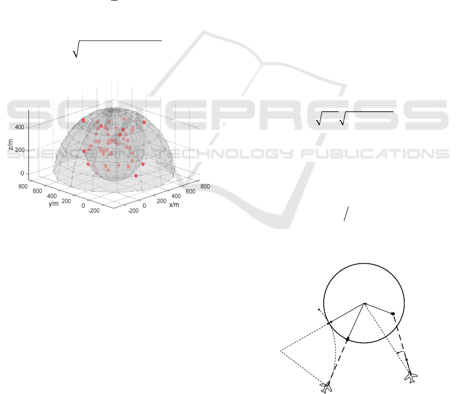
Figure 1: Hemisphere determination from sampling points.
The sphere obtained by this fitting method can’t
cover all sampling points, and the sampling points
can’t represent obstacle completely yet, which is
limited by sensor capabilities. A hemisphere model
slightly larger than the sphere can be determined, the
centre coordinate and radius of hemisphere is the
bottom and twice radius of the sphere, respectively.
The equation of the hemisphere is:
()
()
()
2
2
2
2
(2 ) ,
xyz z
x
oyozorrzor−+−+−−= ≥+
(7)
3 OBSTACLE AVOIDANCE
ALGORITHM BASED ON
OPTIMAL PATH
After pre-processing of obstacles in flight scenes, the
hemisphere obstacle model is obtained. In order to
make the UAV track the predefined waypoints path
without obstacle offending, a novel obstacle
avoidance algorithm based on hemispherical optimal
path is designed, and the avoidance rules are
determined.
3.1 Obstacle Detection and Avoidance
Determination
Design a suitable virtual “line-of-sight”
det
L
according to the aircraft flight performance and
obstacle size, which is a constant and consistent with
aircraft flight direction, it is important to determine if
the aircraft intersects the obstacle. As shown in the
left of Figure 2, the line of sight is the shortest one
when UAV avoids obstacles with the minimum
turning radius, then the minimum detection line
det,min
L
is obtained by Pythagorean theorem as,
det,min obs obs min obs
2
L
RR R R=+−
(8)
Where
obs
R is the radius of the corresponding
hemisphere circle at the local altitude for the aircraft,
min
R
represents the minimum turn radius of the
aircraft and is given,
()
2
min max
tan
n
RVg φ =
(9)
Where
n
V
and
max
φ
are the ground speed and the
maximum roll angle of the UAV, respectively.
det,min
L
obs
R
min
R
det
L
D Δ
a
n
V
O
Figure 2: Obstacle detection geometry logic.
An Innovative Obstacle Avoidance Algorithm for UAV Based on Hemispherical Optimal Path
837

In order to obtain the final value of
det
L
,
additional compensation factors must be considered
for the roll angle delay time
roll
t
, which is from the
initial angle to
max
φ
. Then the delayed distance can
be obtained with
n
V
multiply by
roll
t
, which is added
to
det,min
L
, then
det
L
is given as following,
det det,min rolln
L
LVt=+
(10)
Eq. (11) satisfies as,
det obs
DL R≤+
(11)
Where,
D
is the distance between UAV and the
centre of circle, which means that the UAV starts to
detect the obstacles. As shown in Figure 2, if
obs
aR=
, the end of the detection line is on the edge
of the obstacle, if
obs
aR≤
, the detection line touches
the obstacle, the aircraft needs to avoid flight action
to be away from the obstacle, where
a
is the segment
obtained by the centre of circle and the end of the
detection line.
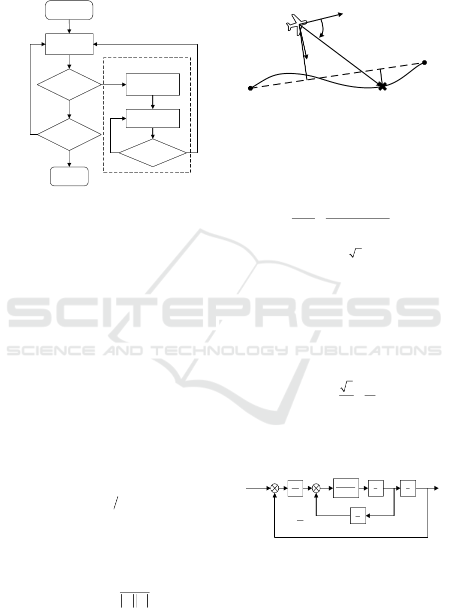
3.2 Optimal Avoidance Path
As depicted in Figure 3,
12
,WP WP
are two waypoints
on target path, the coordinates in the East-North-Up
(ENU) frame are
()
1, 1, 1,
,,
ENU
wp wp wp
and
()
2, 2, 2,
,,
ENU
wp wp wp
, respectively. The spatial straight
line equation of the two waypoints is:
1, 1, 1,
2, 1, 2, 1, 2, 1,
ENU
E
ENNUU
xwp ywp zwp
wp wp wp wp wp wp
−−−
==
−−−
(12)
Suppose the centre coordinate and radius of the
hemisphere are
(, , )
ENU
ccc
and
R
. According to Eq.
(7) and Eq. (12), the intersection points
M
and N of
the straight line and the hemisphere model can be
calculated. Hence, the shortest distance between the
two points on the spherical surface is the inferior arc
through the maximum circle, which passes through
the intersection points
M
and N , and coincides with
the centre of the hemisphere. The parametric equation
for the circle about points
M
, N and centre
c
is given
as:
cos sin
cos sin
cos sin
EE E
NN N
UU U
xc mR nR
yc mR nR
zc mR nR
ρρ
ρρ
ρρ
=+ +


=+ +


=+ +

(13)
Where, the unit vector
(, , )
ENU
mmm=

m
and
(, , )
ENU
nnn=

n
are perpendicular to each other and
perpendicular to the circular normal vector, and
parameter
[0, 2 ]
ρ
π ∈
.
2
WP
1
WP
c
1
T
2
T
Λ
3
T
R
M
N
Figure 3: Obstacle avoidance problem & optimal
avoidance path determination.
When the UAV detects obstacle threat at the point
1
T , the inferior arc

M
N
is calculated in real time,
which is the shortest avoidance path. Then the UAV
completes the obstacle avoidance by tracking the
optimal avoidance path, then the obstacle avoidance
problem is transformed into the path following
problem. To ensure that the UAV can avoid obstacles
safely, set the hemisphere obstacle radius is
safe
()RL+
, where
safe
L
is safe flight distance.
3.3 Avoidance Success Criteria
During the obstacle avoidance fight, the UAV detects
and judges continuously whether the desired
waypoint is reachable. If the desired waypoint is not
in the obstacle, it means that the desired waypoint is
reachable, otherwise it switches to the next waypoint
of the desired waypoint.
We can compute the angle
Λ
to determine
whether avoidance is over, which is the angle
between the segment made by the UAV’s and the next
valid waypoint, and the segment made by the UAV’s
and the centre of the obstacles. As soon as
/2 π Λ≥
at point
3
T
, means that there is a line of sight to the
next valid waypoint. Then the UAV ends the
avoidance flight and flies to the valid waypoint in
straight trajectory.
The avoidance procedure, connecting with the
waypoint guidance procedure, is described in
Figure4.
ISAIC 2022 - International Symposium on Automation, Information and Computing
838

Waypoints and
obstacle data
Detect obs tacles?
Track avoidance
trajectory
End avoidance
Calculate optimal arc
avoidance trajectory
Y
Y
Y
N
N
N
Regular waypoints
tracking
Reach final
waypoint?
End flight
Avoidance Procedure
Figure 4: Waypoints path tracking and obstacle
avoidance procedure.
4 GUIDANCE SYSTEM
The guidance system and obstacle avoidance
algorithm are mainly responsible for generating a set
of maneuver commands to drive the drone as close as
possible to the predefined and avoidance path.
Therefore, the performance of guidance system is
very important to the aircraft.
4.1 Lateral guidance law
The nonlinear guidance law was first implemented on
UAV by Park (Park et al., 2004). The basic principle
of the guidance law is to select a reference point
P
on
the target trajectory, with a fixed distance
1
L away
from the UAV, which is utilized to produce a lateral
acceleration instruction
L
a according to the position
about the reference point and the current the UAV, as
described in Figure 5. The desired lateral acceleration
is:
()
2
1
2sin
Ln
aVL
η
=
(14)
Where
η
is the angle between the UAV ground
speed vector
n
V and the
1
L
line segment vector, can
expression as:
1
1
arcsin
n
n
η
×
=
VL
VL
(15)
1
WP
2
WP
P
η
1
L
n
V
L
a
d
r
d
Figure 5: Lateral guidance law geometry logic.
Literature (Park et al.,2007) shows the following
transfer function between the lateral deviation of the
UAV and the reference point from the nominal
straight line, which describes the response of the
system as:
2
22
()
() 2
n
rnn
ds
ds s
ω
ξ
ωω
=
++
(16)
Where
0.707
ξ
=
,
1
2/
nn
VL ω =
. Note that the
pole location depends on the values
1
L and
n
V , since
1
L is a fixed value, the value of
n
V directly affects the
stability of the system and the gain of the controller.
In order to ensure that the amplitude-frequency
characteristics of the system do not change under
certain disturbances, the value of
n
V is used to adjust
the value of
1
L dynamically, which improves the
tracking accuracy.
1
1
2
,
n
nn
L
LTV T
V
ω
=== (17)
In order to explore the effects of constant
T
affects the system stability, the roll dynamics is
modelled as a first order inertial, the block diagram is
shown in Figure 6.
1
1
roll
Ts+
2
2
T
2
T
1
s
1
s
1
n
L
T
V
=
L
a
d
r
d
Figure 6: Block diagram of guidance law with roll
dynamics.
In Figure 6, the definition
roll
T is the first order
time constant of the roll angle response to roll
commands. A root locus can be constructed for
An Innovative Obstacle Avoidance Algorithm for UAV Based on Hemispherical Optimal Path
839

various values of
T
using the characteristic equation
for the system:
2
2
32
10
22
roll
TT
T
ssTs+++=
(18)
Figure 7: Root locus of characteristic equation.
The root locus of Figure 7 is constructed for
T
={0.5:0.5:5} and
roll
T
={0,1,2,3}, it is clearly shows
that when
0
roll
T =
, there is no inertia element in the
roll angle response, all roots are in the left half plane,
hence, the system is stable and is not affected by the
constant
T
; when
0
roll
T ≠
, if
roll
TT<
, system is
unstable; if
roll
TT=
, system is marginally stable; if
roll
TT>
, system is stable. Therefore it must be
ensured that the constant
T
is always bigger than the
first time order constant
roll
T .
Given the results of the root locus analysis, it is
shown that
T
can be determined at least 3 to 4 times
more than the first time order constant
roll
T to ensure
satisfactory transient response. Substituting Eq.17
into Eq.14 provides the new
L
a is:
()
2sin
Ln
aVT
η
=
(19)
The desired roll angle which can be obtained
according to the kinematics equation of the UAV is,
()
arctan
cL
ag φ =
(20)
In order to solve the problem for non-smoothing
at the waypoint switching, the arc waypoints
switching strategy is designed to deal with the
overshoot problem during the switching waypoints,
also reduces the cross-track error effectively.
As shows in Figure 8, the target path consists of
three waypoints
1
WP ,
2
WP and
3
WP . The turn angle
β
is given as:
()
()
()
12 12
arccos β =⋅


qq qq
(21)
Where
1

q
,
2

q
are the position vectors of
2
WP to
1
WP and
2
WP to
3
WP , respectively.
1
WP
2
WP
A
B
1
q

2
q

min
R
3
WP
β
C
X
Figure 8: Waypoint switching geometry logic.
 Turn centre: The turn centre is determined at the
distance of
min
sin( 2)R
β
from
2
WP on the line
bisecting the turn angle
β
.
 Turn start criterion: The turn start point is at a distance
of
min
tan( 2)R
β
from the
2
WP on the line linking
1
WP to
2
WP . Turning is starting when the cross-
product
×

 
CX CA
changes sign.
 Turn stop criterion: The turn stop point is at the
distance of
min
tan( 2)R
β
from the
2
WP on the
line joining the
2
WP and
3
WP . Turning is ended
when the cross-product
×

 
CX CB
changes sign.
4.2 Altitude Guidance Law
In this paper, taking the 3D path following problem
of the aircraft as horizontal and altitude path tracking,
the horizontal trajectory tracking control signal is the
roll angle obtained by lateral guidance law, and the
altitude tracking control signal is
c
h
can be obtained
as follows:
11
cos tan
c
hhd λ
γ
=+
(22)
Where,
γ
is the flight path angle,
1
d is the
distance from the UAV to the
1
WP under horizontal
projection.
λ is the angle between the segment made
by the UAV’s centre and
1
WP , and the target path
under horizontal projection, as shown in Figure 9.
ISAIC 2022 - International Symposium on Automation, Information and Computing
840

2
WP
1
WP
γ
1
d
λ
1
cosd
λ
1
h
2
h
c
h
Figure 9: Altitude guidance law geometry logic.
5 SIMULATION AND ANALYSIS
In order to verify the effectiveness of the proposed
autonomous obstacle algorithm and guidance
strategy, the numerical simulations are done by a 6-
DOF nonlinear flight dynamics model for a fixed-
wing UAV. The overall aerodynamic parameters of
the aircraft model are described in (Yang et al., 2013).
The restrictions of the UAV are maximum roll angle
max
30 φ =

, maximum pitch angle
max
20 θ =

. Set
the initial position of the UAV is
(0,0,500)m in ENU
coordinate, the cruising speed
50 /Vms=
, and the
initial speed direction is the true north. Unless
otherwise specified, the predefined states of the UAV
in all simulation tests are the same.
5.1 Path Following Simulation
For the path following simulation, the target route
consists of a set of waypoints, and the waypoints
coordinate date in ENU coordinate is listed in Table
1.
Table 1: Waypoints coordinate of path following.
Waypoints Coordinate
(km)
Waypoint
s
Coordinate
(km)
WP1
WP2
WP3
WP4
WP5
WP6
(0,0,0.5)
(2,0,0.6)
(1,3,0.6)
(3,3,0.6)
(7,-1,0.7)
(
9,-1,0.7
)
WP7
WP8
WP9
WP10
WP11
WP12
(10,0,0.7)
(10,2,0.7)
(9,3,0.7)
(7,3,0.7)
(3,-1,0.5)
(
1,-1,0.5
)
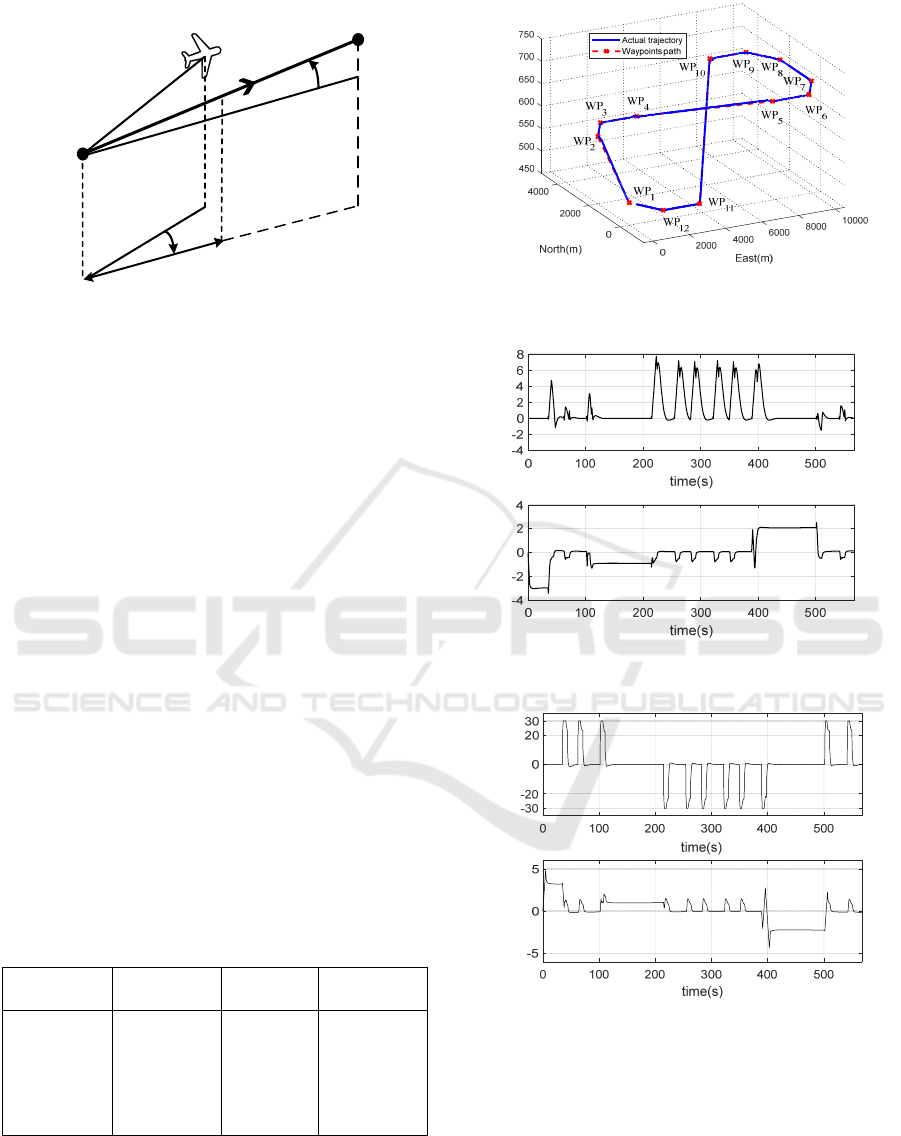
(a)
(b)
(c)
Figure 10: Flight simulation of 3D path following control.
(a) 3D view (b) Euler angle (c) Tracking error.
It can be seen from Figure 10 (a), the UAV tracks
the predefined waypoints path accurately, and
transform waypoints with circular arc path. Figure 10
(c) shows the tracking error during path following,
when the UAV is tracking the path in straight
Up(m)
cross track error(m)height error(m)
roll(deg)
pitch(deg)
An Innovative Obstacle Avoidance Algorithm for UAV Based on Hemispherical Optimal Path
841

segments, the cross track error is almost 0, when the
UAV begins switching waypoints, the error is within
6m±
, and
2.5m±
in tracking circular arc path.
Additionally, the height error is within
4m±
, in a
word, the UAV tracks the whole waypoints path with
small error. Figure 10 (d) shows the Euler angle
response of the UAV, in straight segments, roll angle
response is almost 0, while the UAV tracks the
circular arc path with maximum roll angle in
waypoints switching segment. Similarly, the UAV
has a certain pitch angle response during the climb or
descent, and no response in stable altitude, but due to
the effect of coordinated turn of the UAV in
waypoints switching segments, a certain pitch angle
response will be generated.
5.2 Obstacle Avoidance Simulation
As mentioned in the Sect.2, obstacles can be
modelled by one or more hemispheres. For simple
obstacles, one hemisphere is utilized to cover the
whole or the key parts of the obstacle. For complex
obstacles, the avoidance model can be developed by
multiple cross hemispheres. Before the simulation,
the obstacle hemisphere model has been fitted
according to obstacle data detected by on-board
detection system.
5.2.1 Simple Obstacle Avoidance
For the simple obstacle avoidance simulation, the
UAV faces an obstacle threat during tracking
waypoints path, which intersects with target path. The
pre-defined waypoints coordinate and obstacle date
are listed in Table 2. Set the safe flight distance
safe
100
L
m=
.
Table 2: Waypoints and simple obstacle date.
Waypoints Coordinate(km) Obstacle Date(km)
WP1
WP2
WP3
WP4
(0,0,0.5)
(0,4,0.5)
(1.2,4,0.5)
(
1,0.7,0.5
)
Centre
Radius
(0.5,2,0)
0.9
(a)
(b)
(c)
Figure 11: Flight simulation of simple obstacle avoidance.
(a) 3D view (b) 2D view (c) Relative distance.
As shown in Figure 11, at first, UAV tracks the
predefined waypoints path, and the obstacle is
detected for the first time by on-board detection
system at 21s. Then a shortest circular arc path is
generated according to the geometric relationship
between waypoints path and obstacle model, the
guidance strategy performing maneuver operation
lets the UAV track the optimal avoidance path, and
complete avoidance flight at 47s, after that, UAV flies
Up(m)
1500
2500
0
1000
1500
3500
3000
500
4000
North(m)
East(m)
1000
500
0
-500
2000
Actual trajectory
Waypoints path
WP
1
WP
2
WP
3
WP
4
ISAIC 2022 - International Symposium on Automation, Information and Computing
842

in straight line to the next reachable waypoint and
continues to fly along the target path. Between
119~144s, UAV detects the obstacle threat and
generates optimal circular arc path again, and
performs the second avoidance action to realize
obstacle avoidance. Figure 11 (c) shows the relative
distance between the aircraft and the surface of
obstacle during the whole flight, we can see that UAV
has always been the outside of the obstacle and about
100m away from the obstacle. Therefore, it can be
confirmed that the obstacle avoidance algorithm
designed in this paper can effectively avoid simple
obstacle.
5.2.2 Complex obstacle avoidance
In order to verify the algorithm is also effective for
complex obstacle, there is a complex obstacle
consisted of two hemisphere models between
waypoints path. The waypoints coordinate and
obstacle date are listed in Table 3.
Table 3: Waypoints and complex obstacles date.
Waypoints Coordinate(km) Obstacles Date(km)
WP1
WP2
WP3
WP4
(0,0,0.5)
(0,4,0.5)
(2.2,4,0.5)
(2,0.7,0.5)
Centre1
Centre2
Radius
(0.5,2,0)
(1.5,2.3,0)
0.9
(a)
(b)
(c)
Figure 12: Flight simulation of the complex obstacle
avoidance. (a) 3D view (b) 2D view (c) relative distance.
It can be seen from Figure 12, the UAV detects
two obstacle threats and avoids obstacles successfully
during the flight simulation. The UAV detects and
avoids obstacle Ⅰ&Ⅱ between 21~47s and 133~157s,
respectively, and the UAV has always been the
outside of the obstacle and about 100m away from the
obstacle. The avoidance algorithm can avoid complex
obstacle effectively.
6 CONCLUSIONS
In this paper, a 3D autonomous real-time obstacle
avoidance algorithm based on hemispherical path
optimal is proposed. The main contributions of this
research are as follows.
1) Mathematical model of obstacles with one or
more hemispheres greatly simplifies obstacle
avoidance algorithm design.
2) Transform obstacle avoidance problems into
trajectory tracking problems to realize the
optimal obstacle avoidance trajectory.
3) Design the variable gain virtual reference point
nonlinear guidance law and arc waypoint
switching strategy, which effectively improves
the trajectory tracking accuracy.
4) The 3D trajectory tracking and obstacle
avoidance simulations verify the effectiveness
of the autonomous obstacle avoidance
algorithm, with considering the limitations and
kinematics of the UAV itself, which reveals to a
good applicability in practical engineering.
Beyond that, to accomplish the fundamental
purpose of the UAV trajectory planning and collision
avoidance, (1) the known obstacle model is pre-set in
flight control computer, the drone follows the arc path
relative distance(m)
An Innovative Obstacle Avoidance Algorithm for UAV Based on Hemispherical Optimal Path
843

according to the designed hemispherical convex in
flight experiment; (2) the laser radar is installed on a
drone to collect the obstacle feature points and fit the
model in real time, using to evaluate the accuracy of
the obstacle modelling.
ACKNOWLEDGMENTS
This research was made possible by Fundamental
Research Funds for the Central Universities Grant
No. 56XAC22030.
REFERENCES
Agarwal, D., and Bharti, P. S. (2018). A review on
comparative analysis of path planning and collision
avoidance algorithms. International Scholarly and
Scientific Research & Innovation
, 12(6):608-624.
Ai-kaff, A., García, F., Martín, D., Escalera A. D. L., and
Armingol, J. M. (2017). Obstacle detection and
avoidance system based on monocular camera and size
expansion algorithm for UAVs. Sensors, 17(5):1061-
1082.
Elhoseny, M., Tharwat, A., and Hassanien, A. E. (2018).
Bezier curve based path planning in a dynamic field
using modified genetic algorithm. Journal of
Computational Science
, 25:339-350.
Gochev, M. I., Nadzinski, M. G., and Stankovski, D. M.
(2017). Path planning and collision avoidance regime
for a multi-agent system in industrial robotics.
International Scientific Journal “Machines
Technologies Materials”
,11:519-522.
Ha, L. N. N. T., Bui, D. H. P., and Hong, S. K. (2019).
Nonlinear control for autonomous trajectory tracking
while considering collision avoidance of UAVs based
on geometric relations. Energies, 12:1551-1570.
Hildmann, H., and Kovacs, E. (2019). Review: Using
unmanned aerial vehicles (UAVs) as mobile sensing
platforms (MSPs) for disaster response, civil security
and public safety.
Drones, 59(3):1-26.
Kwasniewski, K. K., and Gosiewski, Z. (2018). Genetic
algorithm for mobile robot route planning with obstacle
avoidance.
Acta Mechanica et Automatica, 12(2):151-
159.
Lacono, M., and Sgorbissa, A. (2018). Path following and
obstacle avoidance for an autonomous UAV using a
depth camera.
Robotics and Autonomous Systems,
106:38-46.
Mairaj, A., Baba, A. I., and Javaid, A. Y. (2019).
Application specific drone simulators: Recent advances
and challenges. Simulation Modelling Practice and
Theory
, 94:100-117.
Park, S., Deyst, J., and How, J. P. (2004). A new nonlinear
guidance logic for trajectory tracking. In 2004 AIAA
Guidance, Navigation, and Control Conference and
Exhibit (GNCCE)
, pages:1-16. AIAA.
Park, S., Deyst, J., and How, J. P. (2007). Performance and
lyapunov stability of a nonlinear path following
guidance method. Journal of Guidance, Control, and
Dynamics
, 30(6):1718-1728.
Radmanesh, M., Kumar, M., Guentert, P. H., and Sarim, M.
(2018). Overview of path-planning and obstacle
avoidance algorithms for UAVs: a comparative study.
Unmanned Systems, 6(2): 95-118.
Sasongko, R. A., Rawikara, S. S., and Tampubolon, H. J.
(2017). UAV obstacle avoidance algorithm based on
ellipsoid geometry.
Journal of Intelligent & Robotic
Systems
, 88(2-4):567-581.
Tang, J., Sun J., Lu, C., and Lao, S. (2019). Optimized
artificial potential field algorithm to multi-unmanned
aerial vehicle coordinated trajectory planning and
collision avoidance in three-dimensional environment.
In
Proceedings of the Institution of Mechanical
Engineers, Part G: Journal of Aerospace Engineering
,
233(16): 6032-4043.
Wan, Y., Tang, J., and Lao, S. (2019). Research on the
collision avoidance algorithm for fix-wing UAVs based
on maneuver coordination and planned trajectories
prediction.
Applied Sciences, 798(9):1-20.
Yang, X., Mejias, L., and Bruggemann, T. S. (2013). A 3D
collision avoidance strategy for UAVs in a non-
cooperative environment.
Journal of Intelligent &
Robotic Systems
, 70:315-327.
Zammit, C., and Erik-Jan, V. K. (2018). Comparison
between A* and RRT algorithms for UAV path
planning. In
2018 AIAA Guidance, Navigation, and
Control Conference(GNCC)
, pages 1-23. AIAA.
Zhang, J., Liu, B., Meng, Z., and Zhou Y. (2018).
Integrated real time obstacle avoidance algorithm based
on fuzzy logic and L1 control algorithm for unmanned
helicopter. In 2018 Chinese Control and Decision
Conference(CCDC)
, pages 1865-1870.
Zhang, J., Yan, J., and Zhang, P. (2018). Fixed-Wing UAV
formation control design with collision avoidance
based on an improved artificial potential field.
IEEE
ACCESS
, 6:78342-78351.
Zu, W., Fan, G., Gao, Y., Ma, Y., Zhang, H., and Zeng, H.
(2018). Multi-UAVs cooperative path planning method
based on improved RRT algorithm. In
2018 IEEE
International Conference on Mechatronics and
Automation (ICMA)
, pages 1563-1567. IEEE.
ISAIC 2022 - International Symposium on Automation, Information and Computing
844