Deep Reinforcing Learning for Trading with T D(λ)

ZiHao Wang and Qiang Gao

Department of Electronic and Information Engineering, Beihang University, Beijing 100191, China

Keywords:

Trading Decision, Reinforcement Learning, Partially Observable Markov Decision Process, TD(λ), Online.

Abstract:

In recent years, reinforcement learning algorithms for ﬁnancial asset trading have been extensively studied.

Since in ﬁnancial markets the state observed by the agent is not exactly equal to the state of the market, which

could affect the performance of reinforcement learning strategies, the trading decision problem is a Partially

Observable Markov Decision Process(POMDP). However, few studies have considered the impact of the de-

gree of Markov property of ﬁnancial markets on the performance of reinforcement learning strategies. In this

paper, we analyze the efﬁciency and effectiveness of Monte Carlo(MC) and temporal difference(TD) methods,

followed by analyze how T D(λ) combines the two methods to reduce the performance loss caused by partially

observable Markov property with the bootstrap parameter λ and truncated horizon h. Then considering the

non-stationary nature of the ﬁnancial time market,we design a stepwise approach to update the trading model

and Update the model online during the transaction. Finally, we test the model on IF300(index futures of

China stock market) data and the results show that T D(λ) performs better in terms of return and sharpe ratio

than TD and MC methods and online updates can be better adapted to changes in the market, thus increasing

proﬁt and reducing the maximum drawdown.

1 INTRODUCTION

Over the past few decades, ﬁnancial trading has been

a widely studied topic, and various trading meth-

ods have been proposed to trade in ﬁnancial markets

such as fundamental analysis (Singhvi, 1988; Abar-

banell and Bushee, 1998), technical analysis (Lim

et al., 2019; Murphy, 1999) and algorithmic trading

(Schwager, 2017; Chan, 2013) and so on. In recent

years, reinforcement learning has been widely applied

in many areas and has achieved remarkable success

in several application ﬁelds, including autonomous

driving (Cultrera et al., 2020; Shalev-Shwartz et al.,

2016), games (Littman, 1994; Vinyals et al., 2019),

resource scheduling (Mao et al., 2016). At the same

time, the technology is increasingly being used in ﬁ-

nancial transactions to generate higher returns (Deng

et al., 2016; Carapuc¸o et al., 2018; Huang, 2018; Lei

et al., 2020; Moody et al., 1998).

Neuneier et al. (Mihatsch and Neuneier, 2002)

combines the Q-learning algorithm in reinforcement

learning with neural networks to make trading deci-

sions. In the process, they modeled the trading pro-

cess as a Markov decision process (MDP), with in-

stantaneous proﬁt as the reward function. Inspired by

DQN in solving game problems, Chien Yi Huang et

al. (Huang, 2018) modeled the trading decision prob-

lem as an MDP process and adopted DQN for the

model to make trading decisions. Stefan Zohren et al.

(Zhang et al., 2020) also modeled the trading decision

problem to MDP and used three reinforcement learn-

ing algorithms to test in a variety of ﬁnancial markets,

and all achieved higher performance than traditional

technical indicator strategies.

The above study defaults that the trading deci-

sion process is an MDP, i.e., the state of the ﬁnan-

cial market environment is observed by the agent is

be Markovian. And the TD method that exploits the

Markov property of the environment is used for train-

ing. However, there are many factors that affect the

price changes of ﬁnancial assets, including economic

development level, money supply, interest rate, inﬂa-

tion level, balance of payments, population structure,

etc. from a macro perspective. Speciﬁc to the price

impact of a single ﬁnancial asset, it includes the com-

pany’s industrial strength, ﬁnancial status, bullish and

bearish behavior of participating traders, and even ﬁ-

nancial news, market sentiment and other factors. Ob-

viously, according to the public data available in the

market, the above effective information affecting the

price of ﬁnancial assets cannot be fully covered. And

the state would be informationally perfect only if it re-

488

Wang, Z. and Gao, Q.

Deep Reinforcing Learning for Trading with TD(Î

z).

DOI: 10.5220/0011953600003612

In Proceedings of the 3rd International Symposium on Automation, Information and Computing (ISAIC 2022), pages 488-494

ISBN: 978-989-758-622-4; ISSN: 2975-9463

 2023 by SCITEPRESS – Science and Technology Publications, Lda. Under CC license (CC BY-NC-ND 4.0)

tained all information about the history and thus could

be used to predict futures as accurately as could be

done from the full history. In this case, the state S

said to have the full Markov property. But in ﬁnan-

cial market environment, the states of agents can not

be Markov but may approach it as an ideal. There-

fore, ﬁnancial asset trading is not a standard Markov

decision process, but a typical partially observable

Markov decision process.

Furthermore, the TD method exploits Markov

property of the environment (Sutton and Barto, 2018),

so the effectiveness of the TD method is poor in the

ﬁnancial market environment that does not fully meet

the Markov property. Although the MC method does

not exploit the Markov property, it can only be used

for non-continuous tasks and can only be updated un-

til the end of the curtain, so the efﬁciency is low and

requires huge training data for training. Therefore, for

ﬁnancial trading problems with high training speed

requirements and tight data, MC method is not appli-

cable.

Recently, some scholars have considered the par-

tially observable Markov property of ﬁnancial mar-

kets. Chenlin et al. (Chen and Gao, 2019) modeled

the transaction decision problem to POMDP and used

LSTM to make the POMDP close to the MDP and

improve the impact of partial observability. Although

some scholars want to improve the performance im-

pact of some observable ﬁnancial markets, no studies

have optimized the RL training method to reduce the

performance degradation caused by partial observ-

ability.

In this paper, to address the above issues, we de-

scribe the trading decisions problem as a POMDP and

acknowledge that the agent cannot fully observe the

information of the ﬁnancial market. At the same time

the T D(λ) method, which combines TD and MC, is

used for training to improve the performance degra-

dation brought by partial observables and to investi-

gate the effects of the bootstrap parameters λ (which

could trade off TD and MC) and the truncated hori-

zon h (which colud regulating the time period of boot-

strap) on performance. At the same time, considering

the non-stationary nature of the ﬁnancial time mar-

ket, in order to be able to adapt the strategy to the

changes of market conditions as much as possible, we

use a stepwise approach to update the strategy and

make the strategy update online in the test set. Ex-

perimental results of our idea on IF300 data show that

the T D(λ) method outperforms the TD and MC meth-

ods, and that online updating avoids generating large

maximum retractions.

2 METHODY

In this section, we model the trading decisions as

POMDP and introducing our settings of RL including

state spaces, action spaces and reward functions, and

describe the RL algorithm used in this paper, PPO.

Then we analyze the characteristics of RL training

methods, TD, MC and T D(λ) method. Finally, we

study how does the bootstrapping parameters λ with

truncated horizon h affect the efﬁciency and effective-

ness of the T D(λ) method.

2.1 POMDP Formalisation

In ﬁnancial markets, security prices are inﬂuenced by

many factors, such as macroeconomic policies and

microeconomic activities, which contain information

about unpredictable events and the trading behavior

of all market participants. Therefore, it is difﬁcult for

an agent to observe the complete information of the

ﬁnancial market and the trading process can be con-

sidered as a POMDP.

POMDP is a generalization of Markov decision

process. The POMDP is proposed mainly because in

realistic environments, the state observed by the in-

telligence is not equal to the full state of the current

environment, which can affect the learning efﬁcient

and effective of reinforcement learning strategies.

Therefor, we model the transaction decision prob-

lem as a POMDP in which the agent interacts with the

environment at discrete time steps. At each time step

t, the agent obtains the observed value of the environ-

ment as the agent state S

. The more historical infor-

mation this state can represent, the higher the degree

of Markovian properties it contains. The agent se-

lects an action A

according to this state, and receives

a reward R

returned by the environment at the next

time step, while the agent enters the next state S

t+1

A trajectory τ = [S

, A

, R

, S

, A

, R

, S

, A

, R

, . ..]

is generated during the interaction of the agent with

the environment. At time step t, the objective of RL

is to maximize the expected return, denoted as G

time t.

∑

k=t+1

k−t−1

(1)

State Space. The characteristics of ﬁnancial markets

are always contained in the historical prices of assets,

and technical indicators are extracted from the charac-

teristics of prices, so this paper not only uses spreads

as the characteristics of the state space but also uses

technical indicators as part of the state space. A list

of our features is below:

• Normalised spread series,

Deep Reinforcing Learning for Trading with TD(Î

489

• Action at t − 1 moment A

t−1

• MACD indicators shows the relationship between

exponential moving averages of security prices on

different time scales.

MACD

= DEA

− DIF

(2)

DIF

= m(p

t−12:t

) − m(p

t−26:t

)

(3)

DEA

= m(DIF

t−9:t

) (4)

m(x

t−n:t

) is an exponentially weighted moving av-

erage of x with time scale n, p

is close price at

time t.

• RSI indicators is overbought (above 80) or over-

sold (below 20) by measuring the recent rise or

fall in contract prices

RSI =

AUL

AUL + ADL

∗ 100% (5)

AUL is sum of the returns from the last n time

steps, ADL is sum of the losses of the last n time

steps. We set the periods n is 20 days. days in our

state representations.

Action Space. A discrete action space is used, a sim-

ple action set {−1, 0,+1}, where each value directly

represents a position, i.e. -1 corresponds to a short

position, 0 to no position and +1 to a long position.

Reward Function. The reward function depends on

proﬁts R

which deﬁned as

= a

− p

t−1

) − bp p

− a

t−1

) (6)

Transaction costs are necessary because transaction

fees and slippage are inevitable in real transactions,

and deﬁning transaction costs in the reward func-

tion is a major advantage of reinforcement learning.

bp(basis point) is a parameter used to calculate trans-

action fees and slippage.

2.2 RL Algorithm

PPO is proposed to solve the problem of perform-

ing one asymptotic update for each data sample ob-

tained from PG interaction with the environment,

and optimizing a “surrogate” objective function using

stochastic gradient ascent. PPO consists of two net-

works: an actor network that outputs the policy and

a critic network that uses the action value function to

measure the goodness of the chosen action in a given

state. We can update the policy network by maximiz-

ing the ”surrogate” objective function.

CLIP

(θ) =

[min(r

(θ)

, clip(r

(θ), 1 − ε, 1 + ε)

)]

(7)

where

is the advantage function deﬁned as:

= δ

+ (γλ)δ

t+1

+ ··· + (γλ)

(T −t+1)

T −1

(8)

= R

+ γV (S

t+1

|ω) −V (S

|ω) (9)

Whereas standard policy gradient methods per-

form one gradient update per data sample(Zoph et al.,

2018), PPO update more times by add r

(θ) which de-

note the probability ratio to the formula

(θ) =

)

old

)

(10)

To compute the advantage functions, we use the

critic network and train the network using gradient

descent minimizing TD-error

L(ω) = E

[(G

−V (S

|ω))

] (11)

There are many methods to calculate the cumula-

tive discount return G

in the current state, such as

MC, TD and T D(λ). Different application scenarios

should choose different calculation methods, because

the efﬁciency and effectiveness of the models differ

between different calculation methods.

2.3 RL Training Methods

2.3.1 Monte Carlo

The Monte Carlo method requires sampling se-

quences from the interaction of the agent with the

environment and solves the reinforcement learning

problem based on the average sample return, which

is deﬁned as follows.

= R

t+1

+ γR

t+2

+ γ

t+3

+ ··· + γ

T −1

(12)

The Monte Carlo method must wait until the end

of the episode to be updated, because only then is

the return known. But some applications have long

episodes, and postponing all learning until the end of

the episode is too slow. The ﬁnancial trading decision

problem is one such task with a long sequence, so the

efﬁciency of MC is lower. However, they may be less

harmed by violations of Markov properties. This is

because they do not update their value estimates based

on the value estimates of subsequent states. In other

words, this is because they do not perform bootstrap.

2.3.2 Temporal Difference

Temporal Difference methods update their estimates

based to some extent on other estimates. They learn a

guess from a guess, which is called bootstrap method.

The formula is as follows

= R

t+1

+ γV

t+1

) (13)

ISAIC 2022 - International Symposium on Automation, Information and Computing

490

TD exploits Markov property, their aim is to ﬁnd

fully correct estimates of the maximum likelihood

model for Markov processes.Therefore, TD is less ef-

fective for non-Markov environments. However the

TD method only needs to wait one time step to up-

date, and it learns from each transition without regard

to what action is subsequently taken, whereas the MC

method must wait until the end of an episode to up-

date. Therefore, the efﬁciency of TD method is better

than MC method.

2.3.3 T D(λ)

T D(λ) methods unify and generalize TD and MC

methods. T D(λ) methods update with λ-return which

utilizes multi-step jackpot with bootstrapping. The

formula is as follows:

= (1 − λ)

T −t−1

∑

n=1

n−1

t:t+n

+ λ

T −t−1

(14)

t:t+n

t+1

+ γR

t+2

+ . . . +

n−1

t+n

+ γ

t+n−1

t+n

)

(15)

The T D(λ) method approximates the MC method

when lambda equals 1, and it approximates the TD

method when lambda equals 0. MC converges slowly

but has better effectiveness with partially observ-

able Markov decision process, while TD converges

quickly but has poor effectiveness with partially ob-

servable Markov decision process. By adjusting boot-

strapping parameter λ it is possible to balance TD and

MC and reduce the performance degradation caused

by partially observable Markov.

However, lambda-returns depend on n-step re-

turns for arbitrarily large n, and thus can be com-

puted only at the end of the episode, as in the MC

method. But, the longer the reward time, the weaker

this dependence becomes, since each delayed step

drops lambdaγ. Then, approximations can be made

by truncating the sequence after some time steps and

replacing subsequent missing rewards with estimates.

Therefore the the truncated horizon h the greater the

proportion of estimated values.

In general, we deﬁne the truncated λ-return for

time t, given data only up to some later horizon, h,

t:h

= (1 − λ)

h−t−1

∑

n=1

n−1

t:t+n

+ λ

h−t−1

0 <= t < h <= T.

(16)

2.3.4 Performance Analysis of TD(λ)

To illustrate the idea of T D(λ) methods could reduce

the impact of performance degradation brought by

partially observable Markov property, we choose dif-

ferent bootstrapping parameter λ and truncated hori-

zon h for the experiment. For these illustrative exam-

ples, we trained the model 2000 times on three years

of historical data, and we consider the average cumu-

lative returns of the ﬁrst 100 epochs as the evaluation

index of efﬁciency , and the average cumulative re-

turns of the last 100 epochs as the evaluation index of

effectiveness. The experimental results are shown in

Figure 1.

As can be seen in 1(a), when considering the efﬁ-

ciency of the model, the more available value of λ is

on the left side because at this time the T D(λ) method

tends to TD method, while when considering the ef-

fectiveness of the model, as can be seen in 1(b), the

more available value of λ is on the right side, because

at this time the T D(λ) method tends to MC method,

but when λ equals to 1, the efﬁciency and effective-

ness drops sharply because T D(λ) methods produce

a pure Monte Carlo, which converge slower and train-

ing iterations 2000 times still for convergence to a bet-

ter position.

When the truncated horizon h is small, the time

period of bootstrap is shorter, the weight of the esti-

mate is larger, and the effectiveness is poorer. As the

ﬁeld of truncated horizon increases, the time period

for performing the bootstrap increases. There is a sig-

niﬁcant change in state during this time period and the

loss generated by this change can propagate and affect

multiple state updates, so the efﬁciency is higher.

3 EXPERIMENTS AND RESULTS

We design experiments to test our ideas. In this sec-

tion, we present the experimental setup. Then the per-

formance of the T D(λ) method, MC and TD methods

are compared.

3.1 Description of Dataset

We use data on IF300, our dataset ranges from 2002 to

2022, which are shown in Figure 2. We use 11 years

of data for training to get the model. We then retrain

our model every 3 years, using 3 years of data to up-

date the parameters. And for the next 3 years, make

the model parameters are ﬁxed or updated online as a

way to perform trading simulations. So in total, our

test set is from 2013 to 2022.

3.2 Training Schemes for RL

In our work, we use the T D(λ) method and con-

sider effectiveness and efﬁciency separately of the re-

Deep Reinforcing Learning for Trading with TD(Î

491

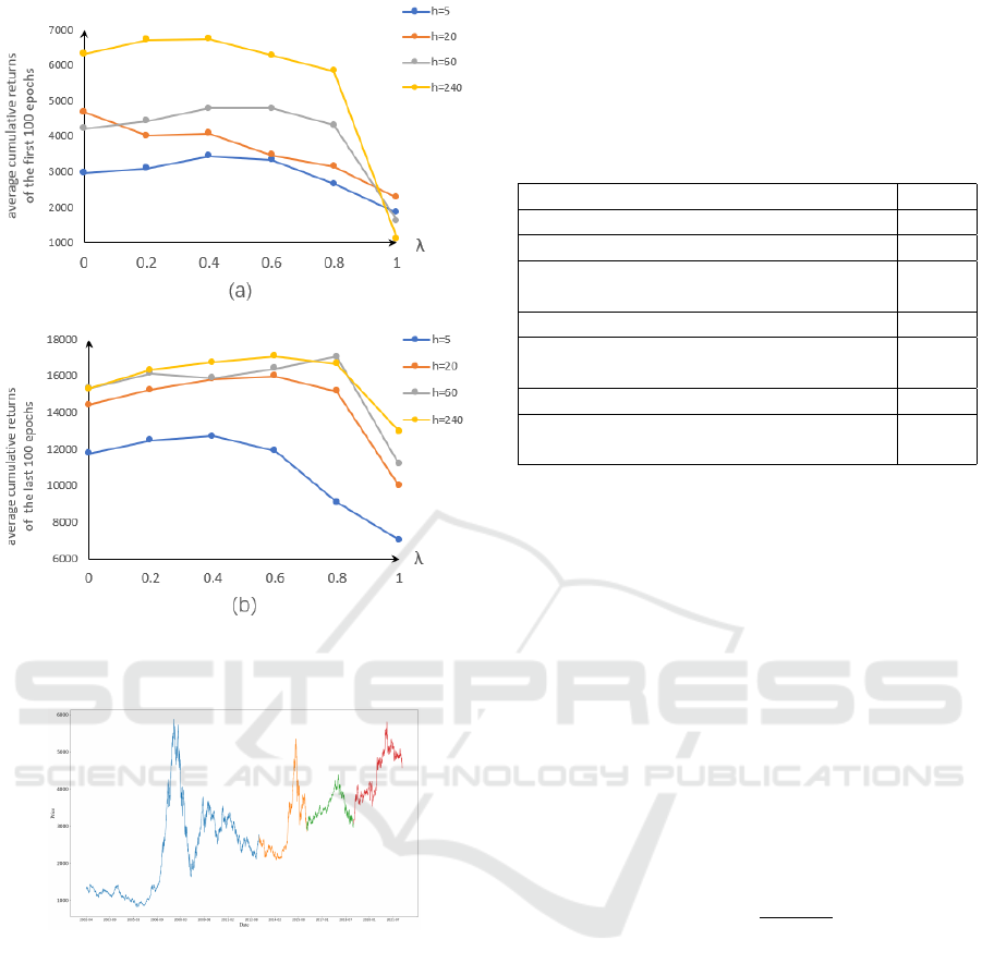
Figure 1: The efﬁciency and effectiveness of T D(λ) varies

with bootstrapping parameter λ and truncated horizon h:(a)

efﬁciency. (b)effectiveness.

Figure 2: Daily closing price of IF300.

inforcement learning strategy and choose different pa-

rameters.

On the train data set, in order to be able to train a

model with the best possible initialization, we chose

the parameters for 6000 training iterations when the

effectiveness of the T D(λ) method was good.

On the test data set, we consider the effectiveness

of the RL methods and retrain our model ofﬂine 2000

times at every 3 years. Model parameters are then

ﬁxed for the next 3 years.

Furthermore, considering the non-stationary na-

ture of the ﬁnancial time market, in order to be able to

adapt the strategy to the changes of market conditions

as much as possible. Model parameters are then up-

dated online for the next 3 years, and in order to avoid

the model training time is long and thus miss timing

of ﬁnancial asset trading, which leads to a large loss,

the parameters of T D(λ) should be chosen when ef-

ﬁciency is better, and the model is updated in the test

set by training 100 epochs in this paper.

Table 1: Values of hyperparameters for different different

methods.

Hyperparameter Value

learning rate α 0.001

discount factor γ 0.99

bootstrapping parameters λ with

efﬁciency

0.2

truncated horizon h with efﬁciency 240

bootstrapping parameters λ with

effectiveness

0.6

truncated horizon h with effectiveness 240

parameter accounting for transaction

fees and slippage bp

3.3 Experimental Results

We test both Buy and Hold and our methods between

2013 and 2022, and We evaluate the performance

of this trading strategy using annualised trade return,

maximum drawdown and Sharpe ratio metrics.

• ER: the annualised trade return focuses on the

proﬁtability of a trading strategy.

ER = E(R

) ∗ 240 (17)

• MDD: the maximum drawdown represents the

maximum loss from any peak in the trading pro-

cess,

MDD = MAX(

− K

),t

< t

(18)

• SR: the annualised Sharpe ratio compares the re-

turn of a trading strategy with its risk.

We show our results in Table 2, where volatil-

ity scaling is used for each method. This allows the

volatility of the different methods to reach the same

target, so we can directly compare these metrics such

as annualised, maximum drawdown and sharpe ratio.

And due to MC only could update until the end of the

curtain, it cannot update online.

Figure 3 illustrates the proﬁt curves for the Buy

and Hold and different RL training methods for the

test period 2013 to 2022. And Buy and Hold refers

to a long position that begins during the test period

and continues through the end of the test period. The

Buy and Hold also represents the change in price of

the IF300.

ISAIC 2022 - International Symposium on Automation, Information and Computing

492

Table 2: Experiment results for the trading strategies volatility targeting.

Trading strategy Update method Method ER MDD Sharpe

ofﬂine

MC 0.288 0.564 0.855

TD 0.284 0.504 0.833

T D(λ) 0.315 0.562 0.937

online

TD 0.296 0.472 0.869

T D(λ) 0.336 0.518 1.003

Buy and Hold / / 0.096 1.013 0.281

Figure 3: The cumulative trade returns for different trading

strategies and methods.

We can see that the RL algorithm provided bet-

ter performance for buy and hold for most of the time

except for the period from May 2014 to June 2015.

This is because the price of the IF300 continued to

rise during this period. Therefore, the smartest trad-

ing strategy in these situations is to hold long posi-

tions and keep them. However, in other periods of

high price volatility, the buy-and-hold strategy per-

formed the worst. the RL algorithm was able to per-

form better in these markets by going long or short at

a reasonable point in time.

Table 2 shows the performance results of Buy and

Hold, and the different RL training methods when up-

date the model ofﬂine and online in the test set quan-

tiﬁcationally. The Buy and Hold has the lower an-

nualised trade return 0.096 than the RL Algorithm.

And the T D(λ) method outperforms both MC and TD

method under ﬁnancial markets with partially observ-

able Markov properties. The annualised trade return

of T D(λ) is 0.315 when update strategy ofﬂine and

0.336 when update strategy online. At the same time,

online updates increase the proﬁtability and decrease

the MDD compared to ofﬂine updates. This is be-

cause the online update allows the strategy to avoid

taking a large-loss action when it encounters a similar

state later in the trading process after experiencing a

large-loss state. These show that online updates allow

better reduce of MDD compared to ofﬂine.

The Sharpe ratio is an indicator that evaluates a

combination of proﬁt and trading risk. It can be seen

from Table 2 that the TD(λ) method when update on-

line has the highest Sharpe ratio (1.003). Therefore,

a good performance in term of the Sharpe ratio is ex-

pected for the T D(λ) method with update online.

4 CONCLUSIONS

In this paper we analyze the speciﬁcity of ﬁnancial

transactions and model the transaction decision pro-

cess as a partially observable Markov decision pro-

cess. We discuss the respective performance charac-

teristics of MC and TD methods and demonstrate that

TD method is more inﬂuenced by the Markov prop-

erties of the environment, and the lower the Markov

property degree, the less effective the strategy model

trained using the TD method is. On the contrary, MC

method is less affected by Markov property, but MC

method puts the learning at the end of the curtain,

so the efﬁciency is poorer. Therefore, in this paper,

we use T D(λ), which combines the two methods, for

testing and analyze the effect of parametric lambda

and truncated horizon h on T D(λ). Considering the

non-stationary nature of the ﬁnancial time market, We

test the model with update online for IF300 data from

2003 to 2022 and verify that the RL strategy outper-

forms the Buy and Hold and that the T D(λ) method

outperforms MC and TD. Furthermore, online up-

dates allow the model to keep up with changes in ﬁ-

nancial market conditions as much as possible.

In the next work, we will investigate adding a fea-

ture extraction model before the RL model and inves-

tigate more technical indicators so that the states can

represent more historical information. Second, differ-

ent reward functions, such as using Sharpe ratio DDL,

are considered so that the model can improve prof-

itability while also considering factors such as risk.

In addition, to further validate the effectiveness of our

model, we will extend the experiment to other mar-

kets, such as stocks, futures, FX, etc.

Deep Reinforcing Learning for Trading with TD(Î

493

REFERENCES

Abarbanell, J. S. and Bushee, B. J. (1998). Abnormal re-

turns to a fundamental analysis strategy. Accounting

Review, pages 19–45.

Carapuc¸o, J., Neves, R., and Horta, N. (2018). Reinforce-

ment learning applied to forex trading. Applied Soft

Computing, 73:783–794.

Chan, E. (2013). Algorithmic trading: winning strategies

and their rationale, volume 625. John Wiley & Sons.

Chen, L. and Gao, Q. (2019). Application of deep reinforce-

ment learning on automated stock trading. In 2019

IEEE 10th International Conference on Software En-

gineering and Service Science (ICSESS), pages 29–

33. IEEE.

Cultrera, L., Seidenari, L., Becattini, F., Pala, P., and

Del Bimbo, A. (2020). Explaining autonomous driv-

ing by learning end-to-end visual attention. In Pro-

ceedings of the IEEE/CVF Conference on Computer

Vision and Pattern Recognition Workshops, pages

340–341.

Deng, Y., Bao, F., Kong, Y., Ren, Z., and Dai, Q. (2016).

Deep direct reinforcement learning for ﬁnancial signal

representation and trading. IEEE transactions on neu-

ral networks and learning systems, 28(3):653–664.

Huang, C. Y. (2018). Financial trading as a game: A

deep reinforcement learning approach. arXiv preprint

arXiv:1807.02787.

Lei, K., Zhang, B., Li, Y., Yang, M., and Shen, Y. (2020).

Time-driven feature-aware jointly deep reinforcement

learning for ﬁnancial signal representation and algo-

rithmic trading. Expert Systems with Applications,

140:112872.

Lim, B., Zohren, S., and Roberts, S. (2019). Enhancing

time-series momentum strategies using deep neural

networks. The Journal of Financial Data Science,

1(4):19–38.

Littman, M. L. (1994). Markov games as a framework

for multi-agent reinforcement learning. In Machine

learning proceedings 1994, pages 157–163. Elsevier.

Mao, H., Alizadeh, M., Menache, I., and Kandula, S.

(2016). Resource management with deep reinforce-

ment learning. In Proceedings of the 15th ACM work-

shop on hot topics in networks, pages 50–56.

Mihatsch, O. and Neuneier, R. (2002). Risk-sensitive re-

inforcement learning. Machine learning, 49(2):267–

290.

Moody, J., Wu, L., Liao, Y., and Saffell, M. (1998). Perfor-

mance functions and reinforcement learning for trad-

ing systems and portfolios. Journal of Forecasting,

17(5-6):441–470.

Murphy, J. J. (1999). Technical analysis of the ﬁnancial

markets: A comprehensive guide to trading methods

and applications. Penguin.

Schwager, J. D. (2017). A Complete Guide to the Futures

Market: Technical Analysis, Trading Systems, Funda-

mental Analysis, Options, Spreads, and Trading Prin-

ciples. John Wiley & Sons.

Shalev-Shwartz, S., Shammah, S., and Shashua, A. (2016).

Safe, multi-agent, reinforcement learning for au-

tonomous driving. arXiv preprint arXiv:1610.03295.

Singhvi, S. (1988). How to make money in stocks: A win-

ning system in good times or bad. Management Re-

view, 77(9):61–63.

Sutton, R. S. and Barto, A. G. (2018). Reinforcement learn-

ing: An introduction. MIT press.

Vinyals, O., Babuschkin, I., Czarnecki, W. M., Mathieu,

M., Dudzik, A., Chung, J., Choi, D. H., Powell, R.,

Ewalds, T., Georgiev, P., et al. (2019). Grandmas-

ter level in starcraft ii using multi-agent reinforcement

learning. Nature, 575(7782):350–354.

Zhang, Z., Zohren, S., and Roberts, S. (2020). Deep rein-

forcement learning for trading. The Journal of Finan-

cial Data Science, 2(2):25–40.

Zoph, B., Vasudevan, V., Shlens, J., and Le, Q. V. (2018).

Learning transferable architectures for scalable image

recognition. In Proceedings of the IEEE conference on

computer vision and pattern recognition, pages 8697–

8710.

ISAIC 2022 - International Symposium on Automation, Information and Computing

494