
State- and Uncertainty-observers-based Controller for a Class of T-S
Fuzzy Models
Hugang Han, Daisu ke Hamasaki and Jiaba o Fu
Graduate School, Prefectural University of Hiroshima, Hiroshima, Japan
Keywords:
T-S Fuzzy Model, State Observer, Uncertainty Observer, Nussbaum-type Function, Adaptive Law, LMIs.
Abstract:
A control system design based on the T-S fuzzy model with uncertainty is considered in this paper. At first,
state observer is developed to estimate the state properly despite the existence of the uncertainty. Then, un-
certainty observer is derived using the estimated state. Finally, a controller based on the observers is proposed
in an effort to counteract the influence of the uncertainty whatever possible. In addition, the Nussbaum-type
function and its relevant properties are used in the controller design to cover the observers’ error and the part
of esti mated uncertainty that is not possibly used through the control matrices. As a result, the closed-loop
control system becomes asymptotically stable.
1 INTRODUCTION
The T-S fuzzy model (Takagi and Sugeno, 1985) is
widely used in the control system design. Because the
consequent of fuzzy rules that compose the T-S fuzzy
model is in the form of the state-space representa tion,
usually the linear system theory can be applied straig-
htforwardly to the T- S fuzz y model-based control sy-
stem design. As a re sult, the co ntrol system stability
will be guaranteed by certain linear matrix inequali-
ties (LMIs), which can be solved by some existing
software packages. Recently, the T-S fuzzy model
has bee n further extended to the so-called polynomial
fuzzy model (Tanaka et al., 200 9; Han et al., 20 17).
However, whatever models ma y be, th ey ar e not more
than a mathe matical description to, usua lly approxi-
mately, describe the dynamics of the concerned sys-
tems. In other words, it seems almost impossible to
form a model immaculately, given that nonlinear sys-
tems are usually considered, and what is more, distur-
bance fr om extern al/internal system, parameters’ per-
turbation and unmodeled dynamics always exist in the
real systems. Such a discre pancy between the concer-
ned system and its model is called uncertainty in this
paper.
The uncertainty may be called different names
such as u nknown input, disturbance in different con-
texts. When it comes to controller desig ns, H
∞
cont-
rol (Wei et al., 2016), adaptive control (Khalil, 2 002;
Han et al., 2001; Liu et al., 2016) are thought to be
very effective ways to dealing with it. Nevertheless,
there is still plenty of room to improve the contr ol per-
formance. For example, when it co mes to H
∞
control
approa c h, the influence of the uncertainty to the state
is no more than being confined to certain prescribed
indexes.
Recently, uncertainty observer-based control pro-
vides a promising approach to handle the uncertainty
and improve robustness. In the existing works (Han,
2016; H an and Lam, 2015), the observers involved are
designed under the assumption that the uncertainty is
not tim e varying. It is clear that such an assumption
is d ifficult to cope with other cases such as acute time
varying uncertainties. Therefore, observing the un-
certainty at a more general level and involving the es-
timated uncertainty in the controller design to cover
its influence as much as possible is the fundamental
notion of this paper. However, at first, a state obser-
ver is presented for the case whe re the state is una-
vailable. Most of state observers based on T-S fuzzy
models in litera ture (Liu and Zhang, 2003; Cao et al.,
2008; Ch adli and Kar imi, 2013; Wei et al., 2016) are
designed in the tr aditional sense similar to the one ba-
sed on the state-space representation, in which some
techniques such as H
∞
approa c h (Cao et al., 2008) and
adaptive contr ol (Lendek et al., 2 010) are used to co-
ver the uncertainty. Inspired by th e existing works for
the case of unknown input (Darouach et al., 1994; Hui
and Zak, 200 5), the one in this paper adopts a different
structure in which some elaborately designed matri-
ces are introduced so that the uncer tainty has no influ-
ence to the the state observer a t all. Then, uncertainty
Han, H., Hamasaki, D. and Fu, J.
State- and Uncertainty-observers-based Controller for a Class of T-S Fuzzy Models.
DOI: 10.5220/0006940305510559
In Proceedings of the 15th International Conference on Informatics in Control, Automation and Robotics (ICINCO 2018) - Volume 1, pages 551-559
ISBN: 978-989-758-321-6
Copyright © 2018 by SCITEPRESS – Science and Technology Publications, Lda. All rights reserved
551

observer is derived using the estimated state. Finally,
a controller based on the o bservers is proposed in an
effort to counteract the influence of the unce rtainty
whatever possible. In addition, the Nussbaum-type
function and its relevant properties are used in the
controller design to cover the observers’ error and the
part of estima te d uncertainty that is not possibly used
through the control matrices; as a result, the closed-
loop control system becomes asymptotically stable .
Throu ghout this paper, M
−
denotes the pseudo-
inverse of M ∈ R
m×n
, i.e., a m atrix satisfying the equa-
tion MM
−
M = M, which means M
−
is either the left
pseudo- inverse M
†
= (M
T
M)
−1
M
T
or right pseudo-
inverse M
‡
= M
T
(MM
T
)
−1
. It is clear that M
†
M = I
n
,
MM
‡
= I
m
. In addition, k · k, and | · | den ote the p-
norm with p being 2, and 1, respectively.
2 STATE AND UNCERTAINTY
OBSERVERS BASED ON T-S
FUZZY MODEL
Assume th a t a nonlinear system can be repre sented by
the following T-S fuzzy model:
Plant Rule i :
If θ
1
(t) is M
i
1
and···and θ
n
θ
(t) is M
i
n
θ
, then
˙x(t) = A
i
x(t) + B
i
u(t) + Dd(t)
y(t) = Cx(t)
(1)
where θ
j
( j = 1, 2, · · · , n
θ
) is a variable in the an te ce-
dent th at is available; M
i
j
(i = 1, 2, . . . , n
r
), a fuzzy
term corresponding to ith rule; x(t) ∈ R
n
, the state
vector; u(t) ∈ R
m
, the input vector; y(t) ∈ R
p
, the out-
put vector; A
i
∈ R
n×n
, B
i
∈ R
n×m
, C ∈ R
p×n
, D ∈ R
n×r
,
some compatible matrices; d(t) ∈ R
r
, uncertainty in-
cluding modeling error, external disturbance , unmo-
deled d ynamics and parameter perturbations. In the
model, it is assumed that rank(CD) = r ank(D).
The overall T-S fuzzy m odel is of the following
form accordingly:
˙x(t) =
∑
n
r
i=1
α
i
(t)
A
i
x(t) + B
i
u(t) + Dd(t)
y(t) = Cx(t)
)
(2)
where θ(t) =
θ
1
(t) θ
2
(t)···θ
n
θ
(t)
,
α
i
(t) =
ω
i
(θ(t))
∑
n
r
i=1
w
i
(θ(t))
≥ 0,
n
r
∑
i=1
α
i
(t) = 1,
ω
i
(θ(t)) =
n
θ
∏
j=1
M
i
j
(θ
j
(t)).
Inspired by the approach of unknown input observer
(UIO), the following state observer is first suggested:
State Observer Rule i :
If θ
1
(t) is M
i
1
and···and θ
p
(t) is M
i
p
, then
˙z(t) = F
i
z(t) + T B
i
u(t) + G
i
y
ˆx(t) = z(t) + Hy(t)
(3)
where z(t) ∈ R
n
, is the in te rnal state vector of the
observer; ˆx(t) ∈ R
n
, the estimate of the state x(t);
F
i
∈ R
n×n
, T ∈ R
n×n
, G
i
∈ R
n×p
, H ∈ R
n×p
, the de-
signs parameters to be determined.
The overall observer of the following form accor-
dingly.
˙z(t) =
∑
n
r
i=1
α
i
(t)
F
i
z + T B
i
u + G
i
y
ˆx(t) = z(t) + Hy(t)
)
(4)
From h ere, unless c onfusion arises arguments
such as t, θ will be omitted just for notational con-
venience.
From (4), we have
˙
ˆx = ˙z + HC ˙x
=
n
r
∑
i=1
α
i
F
i
z + T B
i
u + G
i
Cx + HC(A
i
x + B
i
u + Dd)
=
n
r
∑
i=1
α
i
F
i
z + (T + HC) B
i
u
+(G
i
C + HCA
i
)x + HCDd
. (5)
Defining the estimation error between x and ˆx as:
e
x
= ˆx − x (6)
we have
˙e
x
=
n
r
∑
i=1
α
i
F
i
z + (T + HC)B
i
u + (G
i
C + HCA
i
)x
+HCDd − A
i
x − B
i
u − Dd
=
n
r
∑
i=1
α
i
− (A
i
− G
i
C − HCA
i
)x + F
i
z
+ (T − (I − HC )) B
i
u + (HC − I)Dd
=
n
r
∑
i=1
α
i
(A
i
− G
i
C − HCA
i
)e
x
− (A
i
− G
i
C − HCA
i
) ˆx + F
i
z
+ (T − (I − HC )) B
i
u + (HC − I)Dd
=
n
r
∑
i=1
α
i
(A
i
− G
1i
C − HCA
i
)e
x
− G
2i
Ce
x
− (A
i
− G
i
C − HCA
i
)(z + Hy) + F
i
z
CTDE 2018 - Special Session on Control Theory and Differential Equations
552

+ (T − (I − HC )) B
i
u + (HC − I)Dd
=
n
r
∑
i=1
α
i
(A
i
− G
1i
C − HCA
i
)e
x
− G
2i
C(z + Hy − x)
+ (F
i
− (A
i
− G
1i
C − HCA
i
))z + G
2i
Cz
− (A
i
− G
1i
C − HCA
i
)Hy + G
2i
CHy
+ (T − (I − HC )) B
i
u + (HC − I)Dd
=
n
r
∑
i=1
α
i
(A
i
− G
1i
C − HCA
i
)e
x
+ (F
i
− (A
i
− G
1i
C − HCA
i
))z
+ (G
2i
− (A
i
− G
1i
C − HCA
i
)H)y
+ (T − (I − HC )) B
i
u + (HC − I)Dd
.
(7)
where
G
i
= G
1i
+ G
2i
. (8)
Let
(HC − I)D = 0 (9)
F
i
= A
i
− G
1i
C − HCA
i
(10)
G
2i
= F
i
H (11)
T = I − HC (12)
then we have
˙e
x
=
n
r
∑
i=1
α
i
F
i
e
x
. (13)
Therefore, e
x
converges to zero if F
i
is a Hurwitz ma-
trix as long as th e relations (8)-(12) are held. Now,
let us elaborate on it. From (9), we have HCD = D.
When rank(CD) = rank(D) holds true, CD is a full
column rank ma trix, a solution H of the e quation is:
H = E (CD)
†
. (14)
Once H is determined, G
1i
in (10) can be obtained by
G
1i
= Q
−1
M
1i
(15)
where Q = Q
T
∈ R
n×n
and M
1i
∈ R
n×p
are decision
parameters in the following LMIs that make F
i
a Hur-
witz matrix:
Q > 0 (16)
A
i
Q + QHCA
i
− M
1i
C
+ (A
i
Q + QHCA
i
− M
1i
C)
T
< 0 (17)
for i = 1, 2, ··· , n
r
.
The above L MIs follow from the Lyapunov’s stability
theorem by defining a Lyapunov function V = e
x
Qe
x
.
Finally, having H and F
i
in mind, G
2i
, and T can be
straightfor ward ly obtained from (11), and ( 12), re-
spectively.
After e stablishing the state observer, we move on
to consider how to observe the uncertainty d. As
shown later, there is no necessity to pinp oint d itself,
but the whole term of Dd from the viewpoint of con-
troller design. Letting
D
d
= Dd (18)
an observer of D
d
follows fro m (2):
ˆ
D
d
=
n
r
∑
i=1
α
i
A
i
ˆx + B
i
u
−
˙
ˆx. (19)
Defining the estimation error between D
d
and
ˆ
D
d
as:
e
d
=
ˆ
D
d
− D
d
(20)
it is clear that e
d
→ 0 as long as e
x
→ 0.
In the following, our interest is how to make most
of
ˆ
D
d
in controller design. Considering a special case
of the existence of B
−1
i
, it would be able to design a
controller that is based on a regular control input u
with an extra elemen t such as u − B
−1
i
ˆ
D
d
to counte-
ract the influence of D
d
completely. However, such
a special ca se is h ighly unlikely to happen in the real
system due to the fact that m ≤ n which is the dimen-
sions of th e control matrix B
i
usually. This implies
that
ˆ
D
d
cannot be used in the controller de sig n at this
stage. Nevertheless, we have to diminish the influ-
ence of M
d
whatever possible. For this purpose, let us
recall the fo llowing lemma.
Lemma 1. (Baksalary and Kala, 1979) Let B ∈
R
m×k
, M ∈ R
l×n
, and N ∈ R
m×n
. The equation
BX − MY = N (21)
has a solution X ∈ R
k×n
,Y ∈ R
m×l
, if and only if
I − BB
−
N
I − M
−
M
= 0. (22)
If this is the case, the general solution of (21) has the
form
X = B
−
N + B
−
ZM +
I − B
−
B
W (23)
Y = −
I − B
−
B
NM
−
+ Z −
I − B
−
B
ZMM
−
(24)
where W ∈ R
k×n
, Z ∈ R
m×l
being arbitrary.
It is evident that the condition (22) is held if
M = −I. In this case, (21) admits X = B
−
N an d
Y = −(I = BB
−
)NM
−
as a solution. Therefore, ac-
cording to Le mma 1,
ˆ
D
d
can be divided into the fol-
lowing form:
ˆ
D
d
= B
i
ψ
i
+ ∆E
di
(25)
State- and Uncertainty-observers-based Controller for a Class of T-S Fuzzy Models
553

where ψ
i
= B
†
i
ˆ
D
d
and ∆E
di
=
ˆ
D
d
−B
i
ψ
i
are a solution
of the equation B
i
X +Y =
ˆ
D
d
. By doing so, ψ
i
can be
used in the co ntroller design partially to counteract
the influe nce of D
d
. However, as a solution of the
equation, in fact there is no guarantee that the magni-
tude of ∆E
di
, for example ||∆E
di
||, is less than that of
ˆ
D
d
. In other words, in the case of ||∆E
di
|| > ||
ˆ
D
d
||,
on the contrary, ψ
i
used in the controller design will
worsen the influence of the uncertainty. Therefore, in
order to make sure the effect of the counteraction of
the uncertainty, ψ
i
in (25) is obtained by
ψ
i
=
(
B
†
i
ˆ
D
d
k
ˆ
D
d
− B
i
ψ
i
k ≤ ||
ˆ
D
d
||
0 otherwise.
(26)
From (2 5) we ob serve that ψ
i
shares th e same con-
trol matrix B
i
with the control input u; therefore, it is
the maximum amount to counteract the uncertainty
D
d
from the estimated
ˆ
D
d
. It is clear that ψ
i
= 0 me-
ans that there is no way to use the extracted informa-
tion form
ˆ
D
d
to diminish the influence of D
d
at this
stage. The smaller ||∆E
di
|| is, the better control per-
formance can be expected.
In what follows, let us consider the boundedness
with regard to the estimatio n errors a nd solutions of
equation (25). First, define
Ξ
i j
= (F
i
− A
i
)e
x
− e
d
+ B
i
(ψ
i
− ψ
j
) + ∆E
di
. (27)
In view of the convergence o f e
x
and e
d
along with the
relation in (25), it is clear that Ξ
i j
is bounded.
Let q
i j(k)
(k = 1, 2, ··· , n) be the k-th entr y of the
vector Ξ
i j
∈ R
n
, i.e.,
Ξ
i j
=
q
i j(1)
q
i j(2)
··· q
i j(n)
T
, (28)
and b
i(k)
∈ R
1×m
be the k-th row of B
i
, i.e.,
B
i
=
h
b
T
i(1)
b
T
i(b)
··· b
T
i(n)
i
T
. (29)
Bearing in m ind tha t the boundedness of Ξ
i
in (27), it
is r easonable to a ssume that there exists a scalar κ > 0
such that
max
j=1∼n
r
q
i j(k)
≤ κ · |b
i(k)
|. (30)
In this case, it is easy to che ck that the following ine-
quality holds:
ΓΞ
i j
≤ κ|ΓB
i
| (31)
where Γ ∈ R
1×n
is an arbitrary vector.
Before starting the controller design, we introduce
the Nussbaum-typ e function (Ye and Jiang, 1998) that
is adopted to de sig n a part of controller in compensa-
tion for the influence of Ξ
i j
.
Any continuous function N(ζ) : R → R is a
function of N ussbaum-type functio n if it has the fol-
lowing properties (Nussbaum, 1983):
limsup
z→+∞
1
z
Z
z
0
N(ζ)dζ = +∞ (32)
liminf
z→+∞
1
z
Z
z
0
N(ζ)dζ = −∞ (33)
For example, continuous functions ζ
2
cos(ζ),
ζ
2
sin(ζ) and exp(ζ
2
)cos(
π
2
ζ) are commonly used
as Nussbaum- type functions. Regarding Nussbaum-
type functions, there is the following lemma.
Lemma 2. ( Ye and Jiang, 1998) Let V (·) and ζ(·) be
smooth functions defined on [0,t
f
) with V (t) ≥ 0, ∀t ∈
[0,t
f
), N(·) be even smooth Nussbaum- ty pe function.
If the following inequality holds:
V (t) ≤ c
0
+
Z
t
0
gN(ζ(τ)) + 1
˙
ζ(τ)dτ, ∀t ∈ [0, t
f
)
(34)
where g is a nonzero constant and c
0
repre-
sents some suitable constant, then V (t), ζ(t) and
R
t
0
(gN(ζ(τ)) + 1)
˙
ζ(τ)dτ m ust be b ounded on [0, t
f
).
Also, the following lemma, which is an alternative
to the Barbalat Lemma (Khalil, 2002), will be used in
the system stability analysis later.
Lemma 3. (Ta o, 1997) A function f : R
n
→ R is
square integrable, i.e.,
Z
∞
0
f
T
(t)P f (t)dt < ∞, (35)
where P = P
T
> 0, and has a bounded derivative, then
f (t) → 0, as t → ∞. (36)
3 CONTROLLER DESIGN
Based on the state a nd uncertainty observers, the fol-
lowing controller is proposed.
Controller Rule i :
If θ
1
is M
i
1
and···and θ
p
is M
i
p
, then
u = k
i
ˆx − ψ
i
+ φ
i
(37)
where k
i
∈ R
m×n
is the feedback control gain that
is o btained by k
i
= X
i
Q
−1
with Q = Q
T
> 0 and
X
i
∈ R
m×n
being the d e cision variables of the follo-
wing LMIs:
A
i
Q + B
i
X
j
+ QA
T
i
+ X
T
j
B
T
i
< 0 (38)
for i, j = 1, 2, ··· ,n
r
;
CTDE 2018 - Special Session on Control Theory and Differential Equations
554

ψ
i
is extracted f rom the estimated uncertainty
ˆ
D
d
in
(26) in an e ffort to counteract the influence of the un-
certainty Dd whatever possible; and φ
i
∈ R
m
is desig-
ned in compensation for the influence of Ξ
i j
:
φ
i
=B
T
i
P ˆx + N(ζ)
·
n
r
∑
j=1
α
j
B
T
j
P ˆx + κ · sgn
n
r
∑
j=1
α
j
B
T
j
P ˆx
!!
(39)
where sgn denotes the sign func tion, κ is given in
(30), P = Q
−1
, N(ζ) ∈ R is a Nussbaum-type function
(Nussbaum, 1983), and
˙
ζ =
n
r
∑
i=1
α
i
B
T
i
P ˆx
2
+ κ
n
r
∑
i=1
α
i
B
T
i
P ˆx
. (40)
The overall fuzzy controller (37 ) is of the follo-
wing form acc ordingly.
u =
n
r
∑
i=1
α
i
k
i
ˆx − ψ
i
+ φ
i
. (41)
Substituting (6), (20), (25) and (41) into ( 2), the
closed-loo p control system becomes as follows.
˙x =
n
r
∑
i=1
α
i
A
i
( ˆx − e
x
) + B
i
u +
ˆ
Dd − e
d
=
n
r
∑
i=1
n
r
∑
j=1
α
i
α
j
(A
i
+ B
i
k
j
) ˆx − A
i
e
x
+ B
i
(ψ
i
− ψ
j
)
+ B
i
φ
j
+ ∆E
di
− e
d
. (42)
Substituting (13) and (43) into
˙
ˆx = ˙x + ˙e
x
which fol-
lows from (6), we have
˙
ˆx =
n
r
∑
i=1
n
r
∑
j=1
α
i
α
j
(A
i
+ B
i
k
j
) ˆx − A
i
e
x
+ B
i
(ψ
i
− ψ
j
)
+ B
i
φ
j
+ ∆E
di
− e
d
+ F
i
e
x
=
n
r
∑
i=1
n
r
∑
j=1
α
i
α
j
(A
i
+ B
i
k
j
) ˆx + B
i
φ
j
+ Ξ
i j
(43)
where Ξ
i j
is defined in (27).
Bearing in mind that the relatio n in (13) where F
i
is made to be a Hurwitz matrix, an asymptotically sta-
ble system in (43) does le a d to another asymptotically
stable system in (42). The stability of the system in
(43) is investigated based on the Lyapunov stability
theory. Let us conside r the following quadratic Lya-
punov function candidate:
V = ˆx
T
P ˆx. (44)
Taking the time derivative of V , we have
˙
V =
˙
ˆx
T
P ˆx + ˆx
T
P
˙
ˆx
=
n
r
∑
i=1
n
r
∑
j=1
α
i
α
j
ˆx
T
(A
i
+ B
i
k
j
)
T
P + P(A
i
+ B
i
k
j
)
ˆx
+ 2
n
r
∑
i=1
n
r
∑
j=1
α
i
α
j
ˆx
T
PB
i
B
T
j
P ˆx
+ 2
n
r
∑
i=1
α
i
ˆx
T
PB
i
N(ζ)
·
n
r
∑
j=1
α
j
B
T
j
P ˆx + κ · sgn
n
r
∑
j=1
α
j
B
T
j
P ˆx
!!
+ 2
n
r
∑
i=1
n
r
∑
j=1
α
i
α
j
ˆx
T
PΞ
i j
= − ˆx
T
H ˆx + 2
n
r
∑
i=1
α
i
ˆx
T
PB
i
·
n
r
∑
j=1
α
j
B
T
j
P ˆx + κ · sgn
n
r
∑
j=1
α
j
B
T
j
P ˆx
!!
− 2
n
r
∑
i=1
α
i
ˆx
T
PB
i
· κ · sgn
n
r
∑
j=1
α
j
B
T
j
P ˆx
!
+ 2N(ζ)
˙
ζ+ 2
n
r
∑
i=1
n
r
∑
j=1
α
i
α
j
ˆx
T
PΞ
i j
= − ˆx
T
H ˆx + 2 (1 + N(ζ))
˙
ζ
− 2κ
n
r
∑
i=1
α
i
ˆx
T
PB
i
+ 2
n
r
∑
i=1
n
r
∑
j=1
α
i
α
j
ˆx
T
PΞ
i j
(45)
where
H = −
n
r
∑
i=1
n
r
∑
j=1
α
i
α
j
(A
i
+ B
i
k
j
)
T
P + P(A
i
+ B
i
k
j
)
.
(46)
It is not d ifficult to see that, using (38), H > 0.
Taking the relations (30) and (31) into conside ra-
tion, let us pay attention to the last block in (45).
2
n
r
∑
i=1
n
r
∑
j=1
α
i
α
j
ˆx
T
PΞ
i j
≤2
n
r
∑
i=1
n
r
∑
j=1
α
i
α
j
κ
ˆx
T
PB
i
=2κ
n
r
∑
i=1
α
i
ˆx
T
PB
i
(47)
where the fact that α
i
≥ 0 is used.
Substituting (47) into (45), it follows
˙
V ≤ −ˆx
T
H ˆx +
1 + N(ζ)
˙
ζ (48)
which also implies
˙
V ≤
1 + N(ζ)
˙
ζ (49)
State- and Uncertainty-observers-based Controller for a Class of T-S Fuzzy Models
555

where the fact that H > 0 is used. Integrating (49), it
follows to we get
V (t) ≤ V (0) +
Z
t
0
1 + N(ζ)
˙
ζ(τ)d(τ). (50)
Applying Lemma 2 to (50), we conclude that V (t),
ζ(t), a nd
R
t
0
1 + N(ζ)
˙
ζ(τ)d(τ) must be bounde d.
Again, integrating (48), we have
V (t) ≤V (0) −
Z
t
0
x
T
(τ)Hx(τ)dτ
+
Z
t
0
1 + N(ζ)
˙
ζ(τ)d(τ). (51)
Because V (t) (as well as V (0)) and
R
t
0
1 +
N(ζ)
˙
ζ(τ)d(τ) are all bo unded, it is evident that
R
t
0
ˆx
T
(τ)H ˆx(τ)dτ must be bounded. Therefore , we
conclud e that ˆx (t) is square integrable, and that
lim
t→∞
ˆx(t) → 0 according to Lemma 3.
It is worth no ting that when ψ
i
and φ
i
in (37) are
removed:
u =
n
r
∑
i=1
α
i
k
i
x (52)
reduces to the regular parallel distributed compe n-
sation (PDC) controller (Tanaka and Wang, 2001),
where LMIs in (38) are the stability c onditions for
which the uncertainty Dd in (2) is not considered.
4 SIMULATION
Consider the following altered Van der Pol oscillator:
¨z = −z +
1 − z
2
˙z + u + f
y = 2z + ˙z
(53)
where f denotes uncertainty in the system. In this
simulation, f is assumed to be:
f (t) =
0, if 0 ≤ t < 2
5.3, if 2 ≤ t < 4
0, if 4 ≤ t < 6
−5 + sin(t − 6) + 2 rand(), if 6 ≤ t < 15
3, otherwise
(54)
where rand() is a function that re turns a single uni-
formly random number in the interval (0, 1). T he f
is depicted in Fig. 1. I n the absence of u and f , the
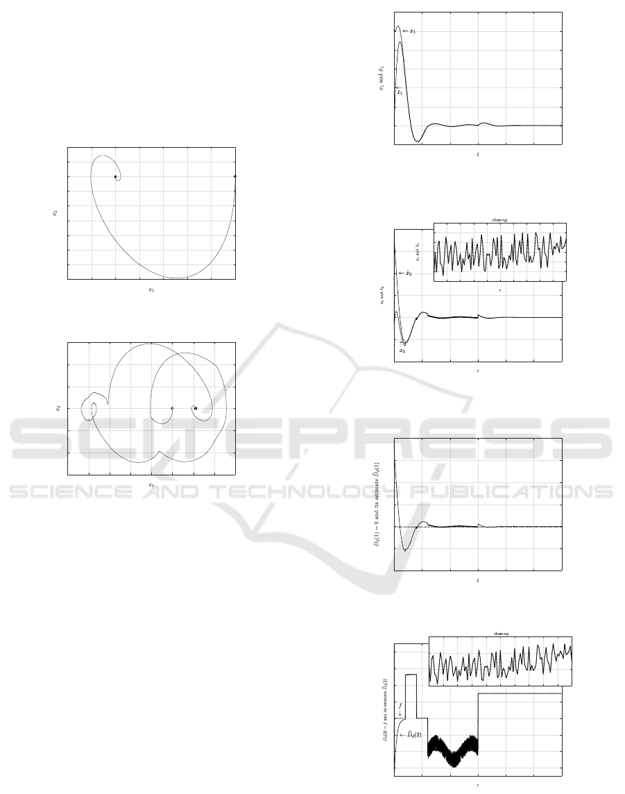
phase plan e z − ˙z is shown in Fig. 2, where the circle
denotes the initial point, the square the end point. It is
clear that the system is unstable without co ntrol.
0 5 10 15 20 25 30
-6
-4
-2
0
2
4
6
Figure 1: Uncertainty f considered in the system (53).
-3 -2 -1 0 1 2 3
-3
-2
-1
0
1
2
3
Figure 2: z − ˙z phase plane with u = 0 and f = 0.
The above nonlinear system can be represented by
the following two-rule T-S fuzzy model:
Rule i : If z is M
i
(z), then
˙x = A
i
x + B
i
u + Dd
y = Cx
(55)
where x
T
= [x
1
x
2
] = [z ˙z], i = 1, 2,
M
1
(z) =
(
9−z
2
9
, −3 ≤ z ≤ 3
0, otherwise
, M
2
(z) = 1 − M
1
(z)
A
1
=
0 1
−1 1
, A
2
=
0 1
−1 −8
, B
1
=
0
1
B
2
= B
1
, C = [
2 1
], D =
0
1
and Dd denotes the uncertainty correspon ding to f in
(53). In this paper, the state x is supposed to be una-
vailable; therefore, instead of z = x
1
in the members-
hip functions, z = ˆx
1
is used in this simulation.
By solving LMIs in (38) with the help of some
software package, k
i
and P = Q
−1
are set to be
k
1
=
−0.4286 −2.0 714
k
2
=
−0.4286 6.92 86
(56)
P =
0.0145 0.0058
0.0058 0.0145
. (57)
A Nussbaum-type function , N(ζ) = ζ
2
cos(ζ) is used
in this simulation. In addition, κ in (39) is set to be
κ = 0.5 + || ˆx||
2
.
CTDE 2018 - Special Session on Control Theory and Differential Equations
556
For comparison purposes, the plant (53) in the ab-
sence o f the uncertainty f is first controlled by the re-
gular PDC controller (52), the contr ol result is shown
in Fig. 3. It is clear that the regular PDC control-
ler is very effective in this case. However, when the
uncertainty in Fig. 1 is applied to the system, as the
control r esult shown in Fig. 4, the regular controller
is no lo nger able to control the system properly.
-0.4 -0.2 0 0.2 0.4 0.6 0.8 1
-0.7
-0.6
-0.5
-0.4
-0.3
-0.2
-0.1
0
0.1
0.2
Figure 3: State driven by the regular PDC controller (52)
without the uncertainty.
-4 -3 -2 -1 0 1 2 3 4
-3
-2
-1
0
1
2
3
Figure 4: State driven by the regular PDC controller (52)
with the uncertainty in (54).
The con trol results by the proposed controller are
shown in Figs. 5∼9. Figs. 5, and 6 depict the re-
sponses of x
1
(dotted line), its estimate ˆx
1
(solid line),
and x
2
(dotted line), its estimate ˆx
2
(solid line), re-
spectively. We observe that the proposed control is
able to make the states of x
1
and x
2
asymptotically
stable, while the state observer (4) is effective to esti-
mate th e real state. Figs. 7, and 8 depict the real un-
certainty D
d
(1) = 0 (dotted line), its estimate
b
D
d
(1)
(solid line), and D
d
(2) = f (dotted line), its e stima te
b
D
d
(2) (solid line), resp ectively. It is evident from
them that
b
D
d
follows D
d
properly. The control input
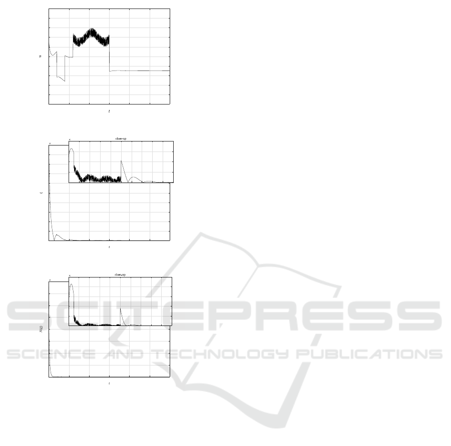
is shown in Fig. 9. In comparison with Fig. 8, control
input u going in the opposite direction to the u ncer-
tainty f acco rdingly is thought to be mainly co ntribu-
ted by ψ
i
that is filtered from
b
D
d
by (25) and (26).
Finally, the behaviors of the other parameters, N(ζ),
ζ, are depicted in Figs. 10, and 11, respectively. It can
be seen that all the parameters involved in the system
are bounded.
0 5 10 15 20 25 30
-0.2
0
0.2
0.4
0.6
0.8
1
1.2
Figure 5: State x
1
and its estimate ˆx
1
driven by the propo-
sed controller (41) along with the observer (4) where the
uncertainty in (54) is applied.
0 5 10 15 20 25 30
-1
-0.5
0
0.5
1
1.5
2
11 11.1 11.2 11.3 11.4 11.5 11.6 11.7 11.8 11.9 12
-0.005
0
0.005
0.01
0.015
0.02
0.025
Figure 6: State x
2
and its estimate ˆx
2
driven by the propo-
sed controller (41) along with the observer (4) where the
uncertainty in (54).
0 5 10 15 20 25 30
-0.01
-0.005
0
0.005
0.01
0.015
0.02
Figure 7: Uncertainty D
d
(1) = 0 (dotted li ne) and its esti-
mate
b
D
d
(1) (solid line).
0 5 10 15 20 25 30
-6
-4
-2
0
2
4
6
8
11 11.1 11.2 11.3 11.4 11.5 11.6 11.7 11.8 11.9 12
-6
-5
-4
-3
Figure 8: Uncertainty D
d
(2) = f (dotted line) as shown in
Fig. 1 and its estimate
b
D
d
(2) (solid line).
State- and Uncertainty-observers-based Controller for a Class of T-S Fuzzy Models
557
0 5 10 15 20 25 30
-10
-8
-6
-4
-2
0
2
4
6
8
10
Figure 9: Control input obtained by (41).
0 5 10 15 20 25 30
0
0.1
0.2
0.3
0.4
0.5
0.6
0.7
0.8
0.9
1
10
-3
5 7 9 11 13 15 17 19 21 23 25
0
2
4
6
8
10
-6
Figure 10: The behavior of ζ.
0 5 10 15 20 25 30
0
0.2
0.4
0.6
0.8
1
1.2
1.4
1.6
10
-6
5 7 9 11 13 15 17 19 21 23 25
0
1
2
3
4
5
10
-11
Figure 11: The behavior of N(ζ).
5 CONCLUSIONS
A design of con trol system based on a class of T-S
fuzzy mod els with uncertainty was considered in this
paper. For the case that the state is unavailable, an
state observer was firstly designed, and then an uncer-
tainty observer was derived using the state estimate.
While it is almost impossible to use the whole esti-
mated uncer ta inty directly in control design, the pa-
per made an effort trying to use it as muc h as possi-
ble to counteract the influence of the unc ertainty. On
the basis of the observers, a controller was proposed ,
in which the Nussbaum- type function and its relevant
properties were used to make the closed-loop system
asymptotically stable.
ACKNOWLEDGEMENTS
The work described in this paper was partially suppor-
ted by JSPS KAKENHI Grant Number JP 16K06189.
REFERENCES
Baksalary, J. K. and Kala, R. (1979). The matrix equation
ax − yb = c. Linear Algebra Appl., 25:41–43.
Cao, Z., Shi, X., and Ding, S. (2008). Fuzzy
state/disturbance observer design for t-s fuzzy sys-
tems with application to sensor fault estimation. IEEE
Trans. Syst. Man Cybern. B Cybern., 38, No. 3:875–
880.
Chadli, M. and Karimi, H. R. (2013). Robust observer de-
sign for unknown inputs takagi-sugeno models. IEEE
Trans. Fuzzy Syst., 21, Issue 1:158–164.
Darouach, M., Zasadzinski, M., and Xu, S. J. (1994). Full-
order observer for linear systems with unknown in-
puts. IEEE Trans. Automa. Contr., 29:606–609.
Han, H. (2016). An observer-based controller for a class
of polynomial fuzzy systems with disturbance. IEEJ
TEEE C, 11, No. 2:236–242.
Han, H., Chen, J., and Karimi, H. R. (2017). State and dis-
turbance observers-based polynomial fuzzy controller.
Information Sciences, 382-383:38–59.
Han, H. and Lam, H. (2015). Polynomial controller de-
sign using disturbance observer. Journal of Advan-
ced Computational Intelligence and Intelligent Infor-
matics, 19, No.3:439–446.
Han, H., Su, C.-Y., and Stepanenko, Y. (2001). Adaptive
control of a class of nonlinear systems with nonline-
arly parameterized fuzzy approximators. IEEE Trans.
on Fuzzy Systems, 9, No. 2:315–323.
Hui, S. and Zak, S. H. (2005). Observer design for systems
with unknown inputs. Intl. J. Appl. Math. Comp. Scie.,
15, No. 4:431–446.
Khalil, H. K. (2002). Nonlinear Systems. Prentice Hall.
Lendek, Z., Lauber, J., Guerra, T., Babuska, R., and Schut-
ter, B. D. (2010). Adaptive observers for ts fuzzy sy-
stems with unknown polynomial inputs. Fuzzy Sets
and Systems, 161, No. 15:2043–2065.
Liu, X. and Zhang, Q. (2003). New approaches to h
∞
con-
troller designs based on fuzzy observers for t-s f uzzy
systems via lmi. Automatica, 39, Issue 9:1571–1582.
Liu, Y.-J., Gao, Y., Tong, S., and Li, Y. (2016). Fuzzy
approximation-based adaptive backstepping optimal
control for a class of nonlinear discrete-ti me systems
with dead-zone. IEEE Trans. on Fuzzy Systems, 24,
Issue 1:16–28.
Nussbaum, R. D. (1983). S ome remarks on a conjecture in
parameter adaptive control. System & Control Letters,
3:243–246.
Takagi, T. and Sugeno, M. (1985). Fuzzy identification of
systems and its applications to modeling and control.
IEEE Trans. Syst., Man, Cybern., 15:116–132.
CTDE 2018 - Special Session on Control Theory and Differential Equations
558

Tanaka, K. and Wang, H. (2001). Fuzzy C ontrol System
Design and Analysis – A Linear Matrix Inequality Ap-
proach. Wiley, New York.
Tanaka, K., Yoshida, H., Ohtake, H., and Wang, H. (2009).
A sum-of-squares approach to modeling and cont-
rol of nonlinear dynamical systems with polynomial
fuzzy systems. IEEE Trans. Fuzzy Syst., 17, No.
4:911–922.
Tao, G. (1997). A simple alternative to the barbalat lemma.
IEEE Trans. Automat. Control, 42, No. 5:698–698.
Wei, X., Wu, Z., and Karimi, H. R. (2016). Disturbance
observer-based disturbance attenuation control for a
class of stochastic systems. Automatica, 63:21–25.
Ye, X. and Jiang, J. (1998). Adaptive nonlinear design wit-
hout a priori knowledge of control direction. IEEE
Trans. Automat. Control, 43, No. 11:1617–1621.
State- and Uncertainty-observers-based Controller for a Class of T-S Fuzzy Models
559
