Optimal Coordination of Robot Motions with Positioner and Linear
Track in a Fiber Placement Workcell
Jiuchun Gao
1
, Anatol Pashkevich
1
, Marco Cicellini
1
and Stéphane Caro
2
1
Laboratoire des Sciences du Numérique de Nantes (LS2N), Institut Mines-Télécom Atlantique, Nantes, France
2
Laboratoire des Sciences du Numérique de Nantes (LS2N), Centre National de la Recherche Scientifique, Nantes, France
Keywords: Redundant Robotic System, Composite Fiber Placement, Optimal Motion Coordination.
Abstract: The paper proposes a methodology for optimal coordination of motions in robotic systems with multiple
redundant actuators. In contrast to our previous results dealing with a single redundant axis, the extended
technique is proposed allowing the robot, positioner and linear track to be actuated simultaneously in order
to reduce the total processing time. The developed technique transforms the original continuous problem
into a discrete one where the desired time-optimal motions are presented as a shortest path on the task graph
satisfying the problem-specific acceleration and velocity constraints imposed on the joint coordinates. The
desired time optimal motions are generated using enhanced dynamic programming algorithm that considers
both of these constraints. Two case studies are presented to demonstrate efficiency of the approach and
evaluate benefits of simultaneous actuation of all robotic system axes.
1 INTRODUCTION
Currently, composite materials have been
increasingly used in aerospace and automotive
industries because of their good strength-to-weight
ratio and durability (Pham et al., 2016, Garoushi,
2018). For fabricating complex composite parts,
automated fiber placement technique is widely used
(Gay, 2014, Frketic et al., 2017). The relevant
technological process can be implemented by using
either specifically designed CNC machines or
robotic systems. Such machines have no limitations
on the component size, but they are expensive and
usually require large work-floor areas (Gallet-
Hamlyn, 2011). In contrast, the robotic systems are
relatively cheap and flexible, allowing changing the
product type easily. However, they are usually
kinematically redundant because of excessive
number of actuated axes that are provided by a 6-dof
robot, a 1-dof positioner and a 1-dof linear track. For
this reason, in robotic fiber placement the optimal
coordination of the manipulator motions with the
positioner/track movements is an important issue.
In literature, there are a number of works that deal
with the redundancy resolution in robotic systems.
Relevant techniques are usually based on the pseudo
inverse of the kinematic Jacobian (Flacco and De
Luca, 2015). However, they can be hardly applied to
the considered problem because they do not allow
generating optimal trajectories satisfying real-life
industrial requirements (Kazerounian and
Nedungadi, 1988). Alternatively, there are also
several techniques based on conversion of the
original continuous problem to a discrete one. The
simplest one is able to generate time-optimal
trajectories for point-to-point motions and was
applied to the spot-welding (Gueta et al., 2008,
Gueta et al., 2017). A slightly different method was
proposed in (Pashkevich et al., 2004) for the laser
cutting and arc-welding applications where the
motion amplitude for the actuated axes was
minimized but the tool speed was assumed to be
constant.
For the considered process, where the tool speed
variations are allowed in certain degree, a discrete
optimization based methodology was proposed in
our previous work (Gao et al., 2017). It allows the
user to convert the original problem to the
combinatorial one taking into account particularities
of the fiber placement technology and to generate
time-optimal coordinated motions for the robot and
positioner. However, the technique was applied to a
planar benchmark example only, with a single
redundant variable. In this work, an extension of the
previous results is proposed allowing dealing with
Gao, J., Pashkevich, A., Cicellini, M. and Caro, S.
Optimal Coordination of Robot Motions with Positioner and Linear Track in a Fiber Placement Workcell.
DOI: 10.5220/0006848105670575
In Proceedings of the 15th International Conference on Informatics in Control, Automation and Robotics (ICINCO 2018) - Volume 2, pages 567-575
ISBN: 978-989-758-321-6
Copyright © 2018 by SCITEPRESS – Science and Technology Publications, Lda. All rights reserved
567

the optimal motion coordination for robotic systems
with higher degree of redundancy, which arises
when the robotic manipulator, the positioner and
linear track actuated simultaneously.
2 ROBOTIC FIBER PLACEMENT
PROBLEM
A typical robotic fiber placement workcell is
presented in Figure 1. Here, the workpiece to be
covered by the composite fiber reinforcement is
manipulated by the positioner, which is able to
change its orientation in order to improve
accessibility of certain zones by the technological
tool. This tool is attached to the robot flange and
ensures placement of the fiber reinforcement in
desired locations. The robot is installed on a
translational linear track allowing adjusting its base
location while processing relative large products.
Figure 1: Robotic fiber placement workcell.
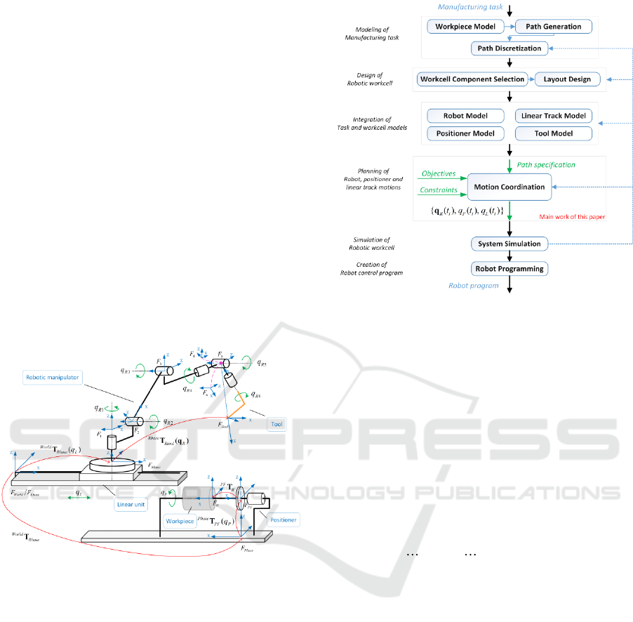
In robot-based composite manufacturing,
preparation of the manufacturing process includes a
number of stages presented in Figure 2, where the
motion coordination of all robotic system
components is one of the most difficult procedures.
Within this process, the desired fiber placement path
is generated using a dedicated CAM system and it is
presented in a discrete form. Further, the obtained
set of task points is transformed into the task graph
that describes all possible combinations of the robot,
positioner and linear track coordinates. Then, the
motion generator produces the optimal trajectories
that correspond to the “shortest” path on the task
graph. Finally, the obtained motions are converted
into the program for the robot control system.
Figure 2: Manufacturing process preparation for robotic
fiber placement processes.
3 SYSTEM KINEMATIC MODEL
To describe the fiber placement task, let us present it
as a sequence of the frames

()
{ , 1,2,... }
i
task
F i n
, in such
a way that the X-axis is directed along the path
direction and Z-axis is normal to the workpiece
surface pointing outside of it. Using these notations,
the task locations can be described by a set of 4×4
homogenous transformation matrices and the
considered task is formalized as follows:
  
(1) ( ) ( )
; 1,2,...
w w i w n
task task task
inTTT
(1)
where all vectors of positions and orientations are
expressed with respect to the workpiece frame (see
superscript “w”). To execute the given fiber
placement task, the technological tool must visit the
frames defined by (1) as fast as possible.
In any task location, the spatial configurations of the
robot, positioner and linear track can be described by
the joint coordinates
R
q
,
P
q
and
L
q
. So, the task
locations can be expressed using the direct kinematic
functions of these components, which are further
denoted as
()
RR
g q
,
()
PP
gq
and
()
LL
gq
. This allows
us to write the kinematic equations describing the
given fiber placement task in the following form
  
   

( ) ( )
( ) ( )
( ) ( )
( ) 1,2,...;
World i i Tool
Lbase L L R R task
World i w i
Pbase P P task
g q g
g q i n
T q T
TT
(2)
where all notations are defined in Figure 1. It is clear
that the above equations cannot be solved for
R
q
,
P
q
ICINCO 2018 - 15th International Conference on Informatics in Control, Automation and Robotics
568

and
L
q
in unique way because the robotic system is
kinematically redundant. On the other side, it gives
some freedom for optimizing the coordinated
motions of the robotic manipulator with the
positioner and linear track movements.
4 GENERATION OF OPTIMAL
COORDINATED MOTIONS
To present the problem in a formal way, let us define
the function
()
R
tq
,
()
P
qt
and
()
L
qt
describing
profiles of the robot, positioner and linear track joint
coordinates as a function of time
[0, ]tT
.
Additionally, let us introduce a sequence of time
instants
12
{ , ,... }
n
t t t
corresponding to the cases when
the technological tool visits the task locations (1).
So, the considered motion coordination problem can
be presented as


   
  


( ), ( ), ( )
()
min max
, , , , , ,
min
, , , ,
{ ( ), ( ), ( ) 1, 2, ... }
min
..
( ( )) ( ( ))
( ( ))
()
()
R L P
R i P i L i
t q t q t
World Tool
Lbase L L i R R i task
World w i
Pbase P P i task
R P L R P L i R P L
R P L R P L i
find
t q t q t i n
such that
T
st
g q t g t
g q t
t
t
q
q
T q T
TT
q q q
qq
 
 



  

























max
,,
min max
, , , , , ,
max
1
()
( ( ))
( ), ( ), ( ) 0
0, ; 1, 2, ...
R P L
R P L R P L i R P L
Ri
R i P i L i
n
t
cond t C
colls t q t q t
where
t t T i n
q
q q q
Jq
q
(3)
where the main objective is to minimize the total
motion time using full capacities of the redundant
robotic system, which are limited by the maximum
velocity/acceleration values for the actuated joints.
Besides, the collision constraints
()colls 
as well as
the distance to singularities
()cond 
are also taken
into account.
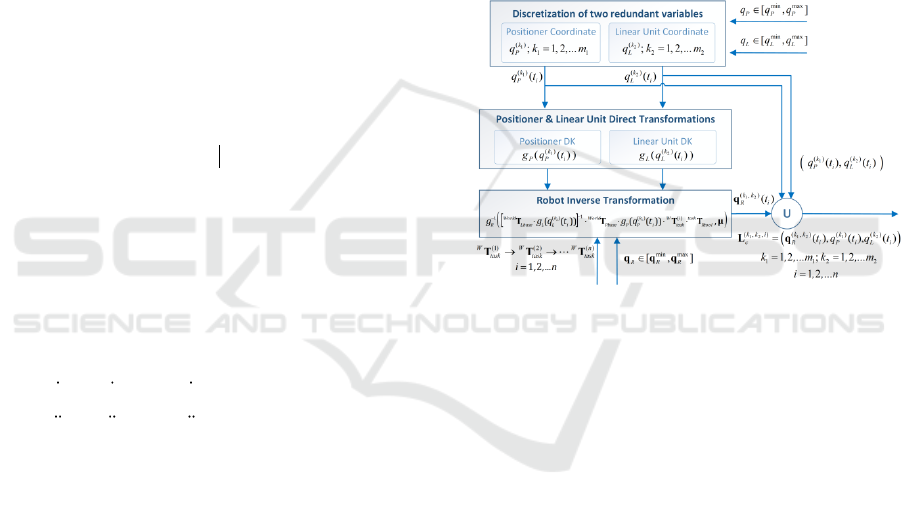
Because of specific constraints, the above presented
continuous optimization problem cannot be solved
in a straightforward way. For this reason, the
considered problem is converted into a discrete form
by sampling the redundant variables corresponding
to the positioner and the linear track. Then, using
ideas proposed in our previous work (Gao et al.,
2017) and applying sequentially the direct
kinematics of the positioner and linear track as well
as the inverse kinematics of the robot, one can get a
configuration state for the robotic system in joint
space (see Figure 3). This allows generating an
extended task graph where all task locations are
ordered in time. This graph contains all possible
configuration states of the considered robotic system
for executing the given fiber placement path, and the
desired time-optimal solution of the relevant
optimization problem is presented as the shortest
path connecting the initial and the final layers. An
outline of the task graph generation algorithm is
presented in Appendix A.
Figure 3: Transformation of the original continuous
problem into discrete form.
The structure of this 3D graph is presented in
Figure 4 where the nodes

12
( , , )
12
{ , };
k k i
task
kkL
correspond to the i
th
task location
()wi
task
T
and the
indices
12
( , )kk
are related to the sampled
coordinates of the positioner and linear track
respectively.
Using such presentation, the original continuous problem
(1) is converted into a specific shortest-path problem on
the graph, where all three successive nodes satisfy the
acceleration constraints and the distances between two
nodes
12
( , , )k k i
task
L
and

12
( , , 1)k k i
task
L
are equal to the technological
tool displacement time from the i
th
to the (i+1)
th
task point,
which is restricted by the maximum velocities and
accelerations of the robot, the positioner and the linear
track. It should be also noted that some of the nodes are
excluded from the graph because of violation of the
collision or singularity constraints as well as the joint
limits. These nodes are marked as “inadmissible” ones in
Figure 4, and they are not connected to any neighbour. So,
the objective function to be minimized (robot motion time)
Optimal Coordination of Robot Motions with Positioner and Linear Track in a Fiber Placement Workcell
569

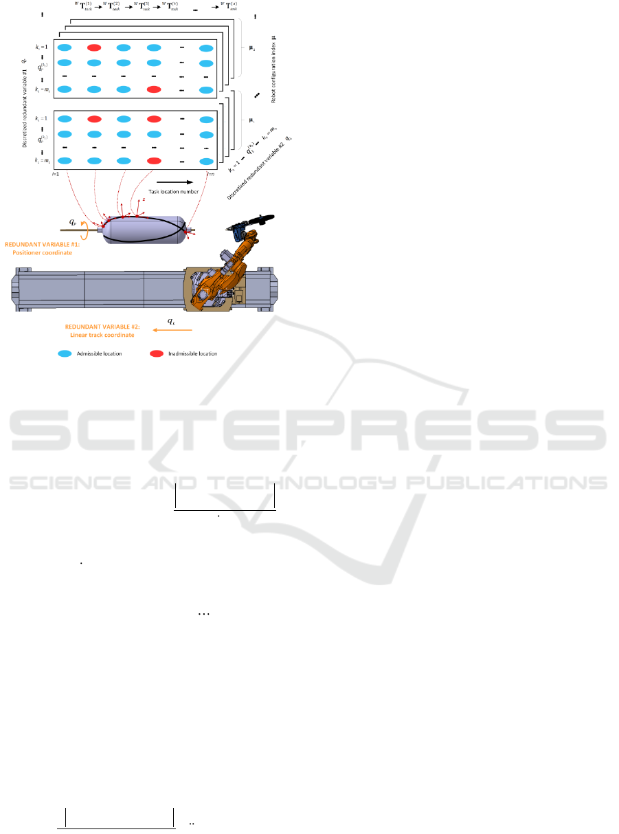
Figure 4: Task graph corresponding to the motion
generation problem with two redundant variables.
can be presented as the sum of the edge weights




 

11
1 2 1 2
( , , ) ( , , 1)
1
1
( , ) min
i i i i
k k i k k i
task task
n
i
T dist LL
(4)
that is computed as












11
1 2 1 2
11
1 2 1 2
( , , ) ( , , 1)
( , , ) ( , , 1)
max
1,2,...8
( , ) max
i i i i
i i i i
k k i k k i
jj
k k i k k i
task task
j
j
qq
dist
q
LL
i.e. taking into account the maximum allowable
velocities

max
{ 1,2,...8};
j
qj
of the actuators.
Corresponding optimal solution is represented by the
sequence

1 1 2 2
1 2 1 2 1 2
( , , 1) ( , , 2) ( , , )
{ } { } { }
nn
k k k k k k n
task task task
L L L
that
contains the actuated coordinates of the robot,
positioner and linear track. It worth mentioning that
the above expression straightforwardly takes into
account the velocity constraints, while the
acceleration constraints are verified by means of the
second order approximation applied to the
corresponding functions
()
R
tq
,
()
P
qt
and
()
L
qt
on
the time interval
11
[ , ]
ii
t t t


. It allows us to present
the acceleration constraints on the desired trajectory
of the considered robotic system in the following
form:
 



    

    
( 1) ( )
1
max
11
2
ii
i j i j
j
i i i i
t q t q
q
t t t t
(5)
where


  
11
1 2 1 2
( , , ) ( , , 1)
()
i i i i
k k i k k i
i
j j j
q q q
and the time
intervals

i
t
are computed as the distance between
the nodes
12
( , , )
ii
k k i
task
L
and


11
12
( , , 1)
ii
k k i
task
L
.
To find the desired optimal path, conventional
optimization techniques can be hardly applied
because of extremely high computing time (Gao et
al., 2017). Besides, these techniques are not able to
take into account the acceleration constraints that are
very essential here. For these reasons, a dedicated
problem-oriented algorithm has been developed for
this problem.
This algorithm is based on the dynamic
programming principle, aiming at sequentially
finding the shortest paths for the problems of lower
dimensions, i.e. from

11
12
( , 1)
12
{ , , }
k , k
task
kkL
to the
current nodes

12
( , )
12
{ , , }
ii
k , k i
task
kkL
. If the length of the
corresponding shortest path is denoted as
12
,,k k i
d
,
then the shortest path for the next locations


12
( , , 1)
12
{ , , }
k k i
task
kkL
can be obtained by combining the
optimal solutions for the previous column



12
( , )
12
{ , , }
k k , i
task
kkL
and the distances between the task
locations with the indices i and i+1,
 
 





 
1 2 1 2
1 2 1 2
,
12
( , , 1) ( , )
, , 1 , ,
min ,
kk
k k i k k , i
k k i k k i task task
d d dist LL
(6)
This expression is applied recursively, starting from
the second layer of the task graph (
2i 
) and
finishing by the last one (
in
). So, the desired
optimal path can be obtained after selection of the
minimum length

12
, , 1k k i
d
corresponding to the last
layer. An outline of this path planning algorithm is
presented in Appendix B. In fact, this algorithm is
generalization of our previous technique that was
developed for motion coordination of the robotic
manipulator and positioner (without linear track). As
follows from relevant study, this algorithm is rather
time efficient in this more complicated case; which
deals with two redundant axes.
5 COMPARISON OF MOTION
COORDINATION STRATEGIES
To demonstrate advantages of the proposed
technique, let us apply it to an industrial problem
that deals with fabrication of a high-pressure
composite vessel. Relevant robotic fiber placement
workcell (see Figure 5) is composed of 6-axis serial
robot KUKA KR210 R3100, 1-axis translational
ICINCO 2018 - 15th International Conference on Informatics in Control, Automation and Robotics
570

linear track KUKA KL2000 and 1-axis rotational
positioner AFPT 550.
For comparison purposes, two cases will be
considered where the robot base is assumed either
fixed or movable by means of the linear track. These
two cases correspond to different degrees of
redundancy provided by the positioner only or by
the positioner together with the linear track. For the
first case, the technique described in our previous
work (Gao et al., 2017) will be applied while the
second case is based on the technique proposed in
this paper.
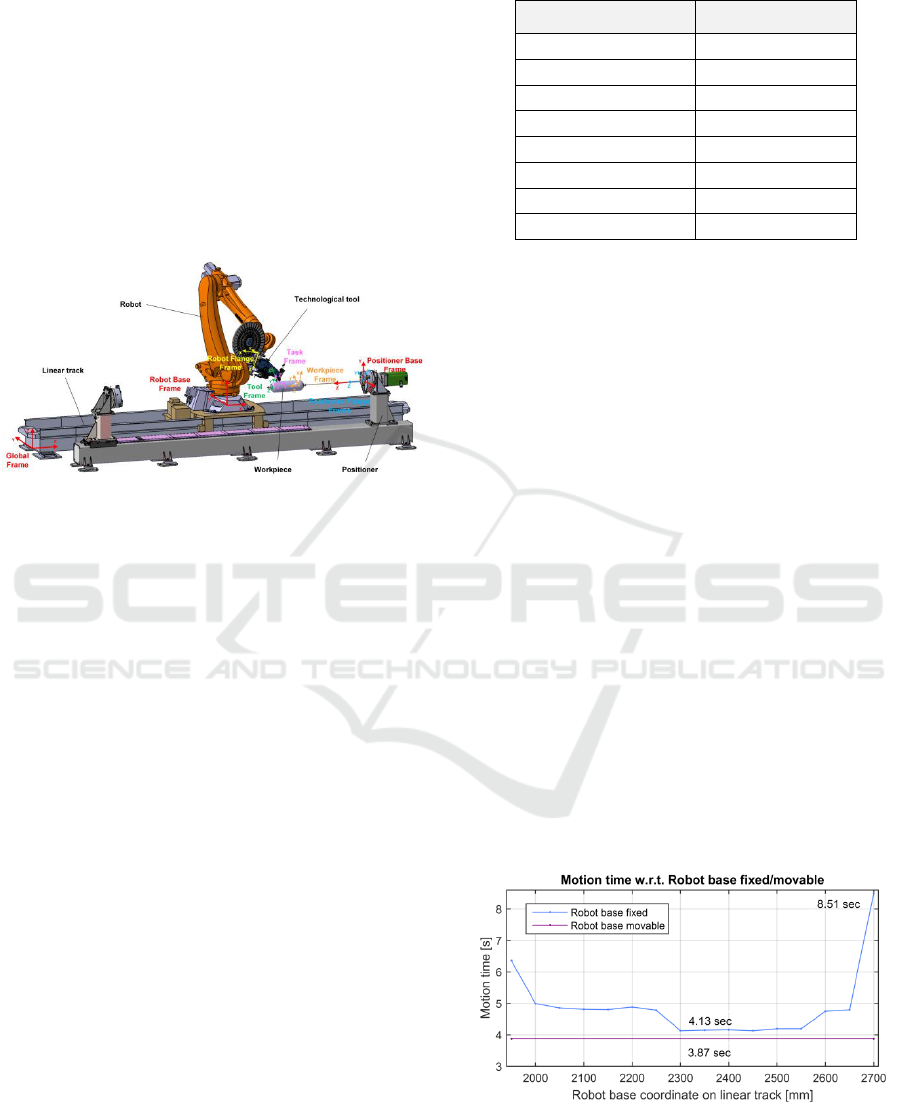
Figure 5: Robot-based fiber placement workcell and
arrangement of coordinate frames.
5.1 Optimal Motion Coordination for
Fixed Robot Base
A composite vessel considered in this case study is
relatively small compared to the robot workspace. It
is composed of a cylindrical part and two elliptical
domes at both ends of the cylinder. The cylinder is
168 mm in diameter and 1200 mm in length. The
laying task includes a single circuit placement of
helical lamina. This allows executing the
manufacturing task with fixed robot base, which
simplifies the motion coordination but obviously
leads to some increase of the total motion time.
Nevertheless, here also arises another optimization
problem that deals with optimal robot placement
relative to the workpiece mounted on the positioner.
To find the optimal location of the robot base, the
space of linear track coordinate (defining the robot
placement) was sampled and the proposed motion
planning technique was applied several times,
assuming that the robot and the positioner
coordination is required only. This yields the 2D
task graph corresponding to a single redundant
variable (positioner rotation angle), which was used
to generate the time-optimal motions for each robot
base location. Relevant results are presented in
Table 1.
Table 1: Total motion time for different robot locations.
Robot location [mm]
Motion time [sec]
2000
4.99
2100
4.80
2200
4.88
2300
4.13
2400
4.16
2500
4.19
2600
4.75
2700
8.51
As follows from the obtained results, the optimal
robot location corresponds to the linear track
coordinate 2300 mm, which ensures the smallest
motion time of 4.13 sec to execute the desired
technological task using capacities of the robot and
the positioner only. It worth mentioning that this
value is about 50% less compared to the non-optimal
robot positioning when the desired path is located
very close to the border of the robot workspace. In
the following section, the obtained motion time will
be compared with the similar value obtained for the
case of movable robot base (when the actuation
capacities of the linear track are also used).
5.2 Optimal Motion Coordination for
Movable Robot Base
Another alternative for manufacturing the
considered composite vessel is to actuate both
positioner and linear track simultaneously, which
corresponds to movable robot base. To coordinate
motions of all mechanical components in this case,
the joint coordinate spaces of both the positioner and
the linear track were sampled with the step of 5° and
15 mm respectively. Then, the proposed extension of
the time-optimal motion generation technique that
deals with two redundant variables was applied.
Figure 6: Total motion time for the cases of non-actuated
and actuated linear track.
Optimal Coordination of Robot Motions with Positioner and Linear Track in a Fiber Placement Workcell
571

Relevant computational results are presented in
Figure 6. As follows from them, using movable
robot base allows reducing the total motion time
down to 3.87 sec, which is about 6% less compared
to the case of the fixed robot base. The obtained
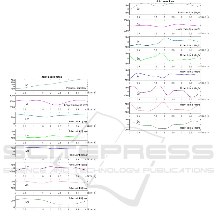
trajectories are shown in Figures 7 and 8, which
show the displacement and velocity profiles for all
eight actuators of the 6-axis robot, 1-axis positioner
and 1-axis linear track. It should be mentioned that
after discrete optimization, a dedicated smoothing
technique may be also used to locally improve the
velocity and acceleration profiles and ameliorate the
actuator working conditions.
Figure 7: Displacement profiles of the coordinated time-
optimal motions of the robot, positioner and linear track.
6 CONCLUSIONS
This paper presents an extended technique dealing with
the optimal motion coordination in redundant robotic fiber
placement systems. In contrast to previous results dealing
with a single redundant axis only, this technique allows
the robot, positioner and linear track to be actuated
simultaneously in order to reduce the total motion time.
First, the original continuous optimization problem is
converted into a combinatorial one where the desired time-
optimal motions are presented as a specific shortest path
Figure 8: Velocity profiles of coordinated time-optimal
motions of the robot, positioner and linear track.
on the task graph. Then, the desired time-optimal
motions are generated using enhanced dynamic
programming algorithm that takes into account the
actuator capabilities (coordinate limits, velocities
and accelerations) as well as the kinematic and
geometric constraints allowing avoiding collisions
and singular configurations of the manipulator. The
proposed technique is illustrated by two case studies
confirming simultaneous actuation of all robotic
system axes. In future, the proposed technique will
be generalized for the robotic systems with higher
degrees of redundancy.
ACKNOWLEDGEMENTS
This work is supported by the China Scholarship
Council (Grant N°210404490018). The author also
acknowledged CETIM for the motivation of this
research work.
REFERENCES
Flacco, F. & De Luca, A. 2015. Discrete-time redundancy
resolution at the velocity level with acceleration/torque
ICINCO 2018 - 15th International Conference on Informatics in Control, Automation and Robotics
572

optimization properties. Robotics and Autonomous
Systems, 70, 191-201.
Frketic, J., Dickens, T. & Ramakrishnan, S. 2017.
Automated manufacturing and processing of fiber-
reinforced polymer (FRP) composites: An additive
review of contemporary and modern techniques for
advanced materials manufacturing. Additive
Manufacturing.
Gallet-Hamlyn, C. 2011. Multiple-use robots for
composite part manufacturing. JEC composites, 28-30.
Gao, J., Pashkevich, A. & Caro, S. 2017. Optimization of
the robot and positioner motion in a redundant fiber
placement workcell. Mechanism and Machine Theory,
114, 170-189.
Garoushi, S. 2018. Fiber-Reinforced Composites. In:
MILETIC, V. (ed.) Dental Composite Materials for
Direct Restorations. Cham: Springer International
Publishing.
Gay, D. 2014. Composite materials: design and
applications, CRC press.
Gueta, L. B., Chiba, R., Arai, T., Ueyama, T., Rubrico, J.
I. U. & Ota, J. 2017. Compact design of a redundant
manipulator system and application to multiple-goal
tasks with temporal constraint. Journal of Advanced
Mechanical Design, Systems, and Manufacturing, 11,
JAMDSM0012-JAMDSM0012.
Gueta, L. B., Chiba, R., Ota, J., Ueyama, T. & Arai, T.
Coordinated motion control of a robot arm and a
positioning table with arrangement of multiple goals.
Robotics and Automation, 2008. ICRA 2008. IEEE
International Conference on, 2008. IEEE, 2252-2258.
Kazerounian, K. & Nedungadi, A. 1988. Redundancy
resolution of serial manipulators based on robot
dynamics. Mechanism and machine theory, 23, 295-
303.
Pashkevich, A. P., Dolgui, A. B. & Chumakov, O. A.
2004. Multiobjective optimization of robot motion for
laser cutting applications. International Journal of
Computer Integrated Manufacturing, 17, 171-183.
Pham, D.-C., Sridhar, N., Qian, X., Sobey, A. J., Achintha,
M. & Shenoi, A. 2016. A review on design,
manufacture and mechanics of composite risers.
Ocean Engineering, 112, 82-96.
APPENDIX A
TASK GRAPH GENERATION
As mentioned in Section 4, here the pseudo-codes of
the 3D task graph generation are presented. Its input
includes is a sequence of 4×4 location matrices
{ ( ) | 1,2,... }Task i i n
, the discretization densities m
1
and m
2
, and the upper/lower limits of the redundant
variables denoted as
max
P
q
,
min
P
q
and
max
L
q
,
min
L
q
respectively. The algorithm transforms the task
locations
()Task i
into the joint space.
This procedure contains two steps. Firstly, the
redundant variables are uniformly discretized in the
ranges of
],[
maxmin
PP
qq
and
],[
maxmin
LL
qq
, and
m
1
×m
2
×n matrix
1 2 1 2
{ ( , , ), ( , , )}
PL
q k k i q k k i
is
obtained, where
1 1 2 2
1,2,... ; 1,2,...k m k m
and
1,2,...in
. Then, at the second step,
(.)
P
g
,
(.)
L
g
and
(.)
1
R
g
are sequentially applied, and the robot
configuration states for
1 2 1 2 1 2
{ ( , , ), ( , , ) | , , }
PL
q k k i q k k i k k i  
are
computed. After checking with the joint limits,
collision and the distance to singularities, the task
graph is finally generated with nodes:
1 2 1 2 1 2 1 2
( , , ) { ( , , ), ( , , ), ( , , )}
P L R
k k i q k k i q k k i k k iLq
where
1 1 2 2
1,2,... ; 1,2,...k m k m
and
1,2,...in
.
Input:
{Task(i)|i=1…n} – matrices of task locations.
{q
P
max
(i), q
P
min
(i)|i=1…n}
– upper/lower limits of positioner coordinate.
{q
L
max
(i), q
L
min
(i)|i=1…n}
– upper/lower limits of linear track coordinate.
m1 – discretization density for positioner.
m2 – discretization density for linear track.
u – robot configuration index.
Output:
{L(k1,k2,i)|k1=1…m1;k2=1…m2;i=1…n}
– 3D matrices of task locations:
Notations:
q
L
, q
P
, q
R
– Linear track, positioner and robot joint
coordinates;
P
T
task
– Transformation from positioner base to task
locations;
R
T
task
– Transformation from robot base to task
locations;
Invoked functions:
g
P
(.) – Positioner direct kinematic function;
g
L
(.) – Linear track direct kinematic function;
g
R
-1
(.) – Robot inverse kinematic function;
coll(.)– Collision test function;
cond(.)– Condition number calculation;
Tran(.)– Transformation from robot base to
positioner base.
Optimal Coordination of Robot Motions with Positioner and Linear Track in a Fiber Placement Workcell
573

APPENDIX B
SHORTEST PATH SEARCH
Here, the pseudo-codes of the shortest path search
are presented. The input is the 3D matrix of the
locations
12
{ ( , , )}k k iL
, which contains information
on the configuration states satisfying the equality
constraint, the collision constraint and the singularity
constraint. The algorithm operates with two tables
( , )D k i
and
( , )P k i
that include the minimum
distances for the sub-problem of lower size (for the
path
1 i
) and the pointers to the previous
locations respectively.
The procedure is composed of four basic steps. The
step (1) reshapes the 3D graph to the one with
m
1
×m
2
lines and n columns for simplifying the
programming. In step (2), the recursive formula (6)
is implemented. For the admissible configuration
nodes, the acceleration constraints are examined
using the expression (5) for each candidate path
connecting the nodes with the indices i, i−1 and i−2.
It is worth mentioning that the function
()accl 
requires three inputs corresponding to i, i−1 and i−2,
but the location for i−2 is determined using the
pointer
( , 1)P j i 
to the previous location in the
current path. Then, it finds the minimum path from
the current node to the first column and records the
reference into the pointer matrix. In steps (3) and
(4), the optimal solution is finally obtained and
corresponding path is extracted by means of the
backtracking.
1) Graph conversion:
m:= m1*m2;
C(k,i):=0; k=1,2,…m; i=1,2,…n;
for i=1 to n
Tem(k1,k2):=0;
for k1=1 to m1
for k2=1 to m2
Tem(k1,k2) = L(k1,k2,i);
end
end
C(:,i):=reshape(Tem);
end
2) Path searching:
set D(k,i):=0;P(k,1):=null;k=1,2,…m;
for i=2 to n
for k=1 to m
for j=1 to m
if(C(k,i)≠null)&(C(k,i-1)≠null)
if(i=2)|(acc(C(k,i),C(j,i-1))=0)
r(j):=D(j,i-1)
+dist(C(k,i),C(j,i-1));
else
r(j):=inf;
end
end
end
set D(k,i):=min({r(j)|j=1,2…m});
P(k,i):=argmin({r(j)|j=1,2…m});
end
end
3) Shortest path selection:
set D
MIN
:=min({D(k,n)|k=1,2,…m});
k
0
(n):=argmin({r(j)|j=1,2…m});
4) Backtracking:
for i=n to 2
k
0
(i-1):=P(k
0
(i),i);
end
Input:
{L(k1,k2,i)|k1=1…m1;k2=1…m2;i=1…n}
– 3D matrix of task locations
Output:
D
MIN
– minimum path length;
{k
0
(i)|i=1…n} – optimal path indices;
Notations:
{D(k,i)|k=1…m1·m2;i=1…n}
– distance matrix;
{P(k,i)|k=1…m1·m2;i=1…n}
– pointer matrix;
{C(k,i)|k=1…m1*m2;i=1…n}
– 2D matrix of task locations;
Invoked functions:
reshape(.)-transform m1×m2 matrix to one
column array;
dist(.) – distance between nodes;
accl(.) - Acceleration test on nodes.
Positioner and linear track discretization:
for i=1 to n
dq
P
(i):=(q
P
max
(i)-q
P
min
(i))/(n-1);
dq
L
(i):=(q
L
max
(i)-q
L
min
(i))/(n-1);
for k1=1 to m1
for k2=1 to m2
q
P
(k1,k2,i):=q
P
min
(i)+(k1-1)·dq
P
(i);
q
L
(k1,k2,i):=q
L
min
(i)+(k2-1)·dq
L
(i);
end
end
end
Location matrix creation:
for i=1 to n
for k1=1 to m1
for k2=1 to m2
P
T
task
:=g
P
(q
P
(k1,k2,i))·Task(i);
R
T
task
:=Tran(q
L
(k1,k2,i))·
P
T
task
;
q
R
(k1,k2,i):= g
R
-1
(
R
T
task
,u);
end
end
end
ICINCO 2018 - 15th International Conference on Informatics in Control, Automation and Robotics
574

The above presented algorithm has been tested using
Matlab 2016b environment (running at Intel
®
i5 CPU
@2.67GHz 2.67GHz). In the case of the fixed robot
base, it took about one minute to generate the time-
optimal motions for each sampled robot location. In
the case of the movable robot base, the computation
required about one hour. It is clear that in other
programming environment, the computing time
would be essentially smaller.
Optimal Coordination of Robot Motions with Positioner and Linear Track in a Fiber Placement Workcell
575