Colorectal Cancer Classiﬁcation using Deep Convolutional Networks

An Experimental Study

Francesco Ponzio, Enrico Macii, Elisa Ficarra and Santa Di Cataldo

Department of Control and Computer Engineering, Politecnico di Torino, Corso Duca degli Abruzzi 24, 10129 Torino, Italy

Keywords:

Colorectal Cancer, Histological Image Analysis, Convolutional Neural Networks, Deep Learning, Transfer

Learning, Pattern Recognition.

Abstract:

The analysis of histological samples is of paramount importance for the early diagnosis of colorectal cancer

(CRC). The traditional visual assessment is time-consuming and highly unreliable because of the subjectivity

of the evaluation. On the other hand, automated analysis is extremely challenging due to the variability of

the architectural and colouring characteristics of the histological images. In this work, we propose a deep

learning technique based on Convolutional Neural Networks (CNNs) to differentiate adenocarcinomas from

healthy tissues and benign lesions. Fully training the CNN on a large set of annotated CRC samples provides

good classiﬁcation accuracy (around 90% in our tests), but on the other hand has the drawback of a very

computationally intensive training procedure. Hence, in our work we also investigate the use of transfer

learning approaches, based on CNN models pre-trained on a completely different dataset (i.e. the ImageNet).

In our results, transfer learning considerably outperforms the CNN fully trained on CRC samples, obtaining

an accuracy of about 96% on the same test dataset.

1 INTRODUCTION

Colorectal carcinoma (CRC) is one of the most dif-

fused cancers worldwide and one of the leading

causes of cancer-related death. According to recent

epidemiological data, this type of cancer has signiﬁ-

cant burden in most of the European countries, and it

is still associated with very high mortality rates (Mar-

ley and Nan, 2016). Hence, the early diagnosis and

differentiation of the tumour is crucial for the survival

and well-being of a large number of patients.

Traditionally, pathologists perform CRC diagno-

sis by visually examining under the microscope the

resected tissue samples, ﬁxed and stained by means

of Hematoxylin and Eosin (H&E). The presence and

level of malignancy is assessed by observing the or-

ganisational changes in the tissues, which are high-

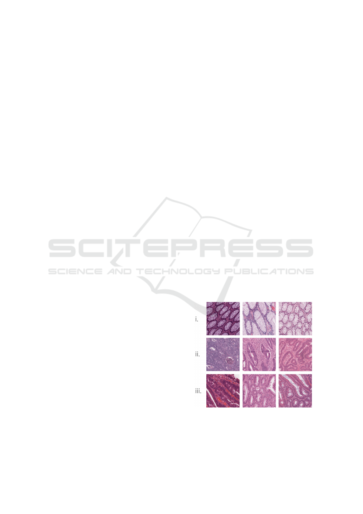
lighted by the two stains. As shown in Figure 1, nor-

mal colon tissues have a well-deﬁned organisation,

with the epithelial cells forming glandular structures

and the non-epithelial cells (i.e. stroma) lying in be-

tween these glands. The main benign precursor of

CRC, adenoma, is characterised by enlarged, hyper-

chromatic and elongated nuclei arranged in a typically

stratiﬁed conﬁguration. Compared to normal tissues,

the adenoma is characterised by either tubular or vil-

lous (ﬁnger-like) tissue architecture. Adenocarcino-

mas, on the other hand, produce abnormal glands that

inﬁltrate into the surrounding tissues.

As it is widely pointed out by literature, manual

examination has two major drawbacks. First, it is

time-consuming, especially for large image datasets.

Figure 1: Histological H&E images of colorectal tissues

(cropped patches). i) Healthy tissue; ii) Adenocarcinoma;

iii) Tubulovillous adenoma.

Second, it is highly subjective and affected by

Ponzio, F., Macii, E., Ficarra, E. and Cataldo, S.

Colorectal Cancer Classiﬁcation using Deep Convolutional Networks - An Experimental Study.

DOI: 10.5220/0006643100580066

In Proceedings of the 11th International Joint Conference on Biomedical Engineering Systems and Technologies (BIOSTEC 2018) - Volume 2: BIOIMAGING, pages 58-66

ISBN: 978-989-758-278-3

variability, both inter and intra observer (A. Young

and Kerr, 2011). Hence, there are growing efforts

towards the development of computer-aided diagnos-

tic techniques, with two major directions: (i) auto-

mated segmentation, aimed at partitioning the hetero-

geneous colorectal samples into homogeneous (i.e.

containing only one type of tissue) regions of inter-

est. (ii) automated classiﬁcation, aimed at categoris-

ing the homogeneous tissue regions into a number of

classes, either normal or malignant, based upon quan-

titive features extracted from the image. In both the

tasks, the main challenge to be tackled is the extreme

intra-class and inter-dataset variability, that is an in-

herent characteristic of histological imaging. In this

work, we focus on the automated classiﬁcation task,

and speciﬁcally into three histological categories that

are most relevant for CRC diagnosis: (i) healthy tis-

sue, (ii) adenocarcinoma, (iii) tubulovillous adenoma.

In the last few years, the literature on automated

classiﬁcation of histological images has been exten-

sive, with applications covering different anatomical

parts other than colon, such as brain, breast, prostate

and lungs. Most of the proposed approaches rely on

automated texture analysis, where a limited set of

local descriptors are computed from patches of the

original input images and then fed into a classiﬁer.

Among the most frequently used, statistical features

based on grey level co-occurrence matrix (GLCM),

local binary patterns (LBP), Gabor and wavelet trans-

forms, etc. The texture descriptors, eventually en-

coded into a compact dictionary of visual words, are

used as input of machine learning techniques such

as Support Vector Machines (SVM), Random Forests

or Logistic Regression classiﬁers (Di Cataldo and Fi-

carra, 2017). In spite of the good level of accuracy

obtained by some of these works, the dependence on

a ﬁxed set of handcrafted features is a major limita-

tion to the robustness of the classical texture analysis

approaches. First, because it requires a deep knowl-

edge of the image characteristics that are best suited

for classiﬁcation, which is not obvious. Second, be-

cause it puts severe constraints to the generalisation

and transfer capabilities of the proposed classiﬁers,

especially in presence of inter-dataset variability.

As an answer to such limitations, in the recent

years the use of deep learning (DL) architectures,

and more speciﬁcally Convolutional Neural Networks

(CNNs), has become a major trend (Janowczyk and

Madabhushi, 2016; Korbar et al., 2017). In CNNs

a number of convolutional and pooling layers learns

by backpropagation a set of features that are best for

classiﬁcation, thus avoiding the extraction of hand-

crafted texture descriptors. Nonetheless, the necessity

of training the networks with a huge number of in-

dependent histological samples is still an open issue,

which limits the usability of the approach in the ev-

eryday clinical setting. Transfer learning (i.e applying

CNNs pre-trained on a different type of images, for

which large datasets are available) seems a promising

solution to this problem (Weiss et al., 2016) but not

fully investigated for CRC classiﬁcation.

In this work. we evaluate a CNN-based ap-

proach to automatically differentiate healthy tissues

and tubulovillous adenomas from cancerous samples,

which is a challenging task in histological image anal-

ysis. For this purpose, we fully train a CNN on a large

set of colorectal samples, and assess its accuracy on

an independent test set. This technique is experimen-

tally compared with two different transfer learning

approaches, both leveraging upon a CNN pre-trained

on a completely different image dataset. The ﬁrst ap-

proach uses the pre-trained CNN to extract a set of

discriminative features that will be fed into a sepa-

rate Support Vector Machines classiﬁer. The second

approach ﬁne-tunes on CRC histological images only

the last stages of the pre-trained CNN. By doing so,

we investigate and discuss the transfer learning capa-

bilities of CNNs in the domain of colorectal tissues

classiﬁcation.

2 MATERIALS AND METHODS

2.1 Colorectal Cancer Image Dataset

The dataset used in this study was extracted from

a public repository of H&E stained whole-slide im-

ages (WSIs) of colorectal tissues, available on line

at http://www.virtualpathology.leeds.ac.uk/. All the

slides are freely available for research purposes, to-

gether with their anonymised clinical information.

In order to obtain a statistically signiﬁcant dataset

in terms of inter-subjects and inter-class variability,

27 WSIs were selected among univocal subjects (i.e.

one WSI per patient). Note that different types of tis-

sues (e.g. healthy and cancerous portions) coexist in a

single WSI. With the supervision of a skilled pathol-

ogist, we identiﬁed large regions of interest (ROIs)

on the WSIs as in the example of Figure 3, so that

each ROI is univocally associated to one out of the

three tissue subtypes: (i) adenocarcinoma (AC); (ii)

tubuvillous adenoma (TV) and (iii) healthy tissue (H).

Then, the ROIs were cropped into a total number of

13500 1089x1089 patches (500 per patient), at a mag-

niﬁcation level of 40x.

For training and testing purposes, the original

image cohort was randomly split into two disjoint

subsets, comprising 18 subjects for training (9000

Colorectal Cancer Classiﬁcation using Deep Convolutional Networks - An Experimental Study

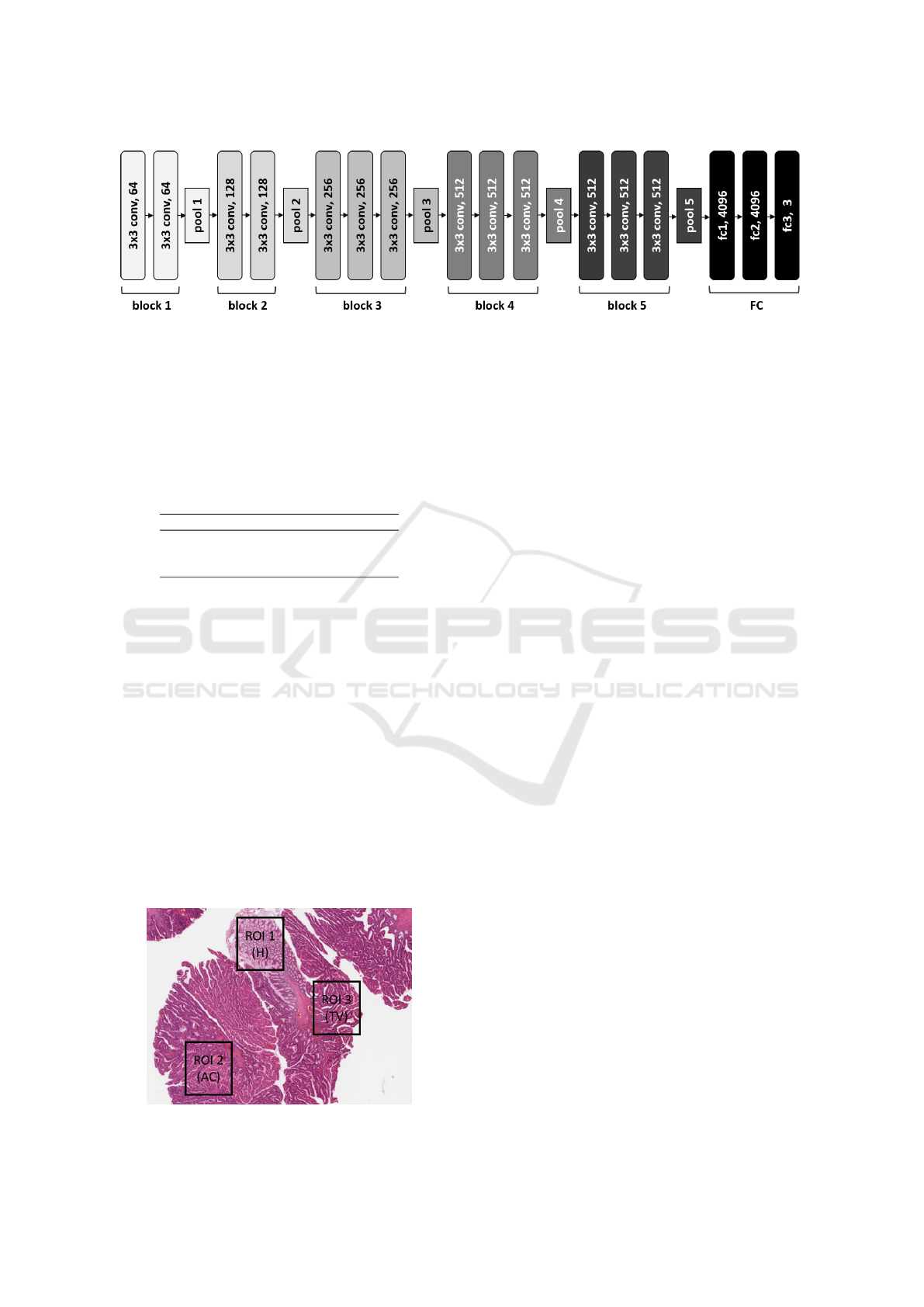
Figure 2: CNN architecture.

patches in total) and 9 for testing (4500 patches). See

Table 1 for a complete characterisation of the two sets.

The random sampling was stratiﬁed, so that both the

training and the testing dataset are balanced among

the three classes of interest (H, AC and TV, respec-

tively).

Table 1: CRC image dataset.

Train Test Tot

# of patients 18 9 27

# of ROIs 85 24 109

# of patches 9000 4500 13500

Before being fed into the CNN, each patch was

down sampled by a factor ﬁve, which was empirically

set as a trade-off between computational burden of the

processing and architectural detail of the images. In

order to compensate for the color inconsistencies, the

patches were normalised by mean and standard devi-

ation, computed over the whole training dataset.

2.2 Convolutional Neural Network:

Architecture and Training

Paradigm

A Convolutional Neural Network (CNN) is made up

of multiple locally connected trainable stages, piled

one after the other, with two or more fully-connected

layers as the last step. The ﬁrst part of the network

Figure 3: Identiﬁcation of ROIs from a WSI: example.

is devoted to learning the image representation, with

successive layers learning features at a progressively

increasing level of abstraction, while the last fully-

connected part is devoted to classiﬁcation and acts

like a traditional multilayer perceptron.

From a computational point of view, a CNN archi-

tecture is characterised by two main types of building

blocks:

(i) Convolutional (CONV) blocks, that perform

a 2D convolution operation (i.e. kernel ﬁlter-

ing) on the input image and apply a non-linear

transfer function, such as Rectiﬁed Linear Unit

(ReLU). Based on the trainable parameters of

the kernels, the stage detects different types of

local patterns on the input image.

(ii) Pooling (POOL) blocks, that perform a non-

linear down-sampling of the input (e.g. by ap-

plying a max function). This has the double ef-

fect of reducing the amount of parameters of the

network to control overﬁtting and of making the

image representation (i.e. the local pattern de-

scriptors learnt by the network) spatially invari-

ant.

The number of CONV and POOL blocks (i.e. the

depth) of the network is directly related to the level

of detail that can be achieved in the the hierarchical

representation of the image. Nonetheless, a higher

depth also translates into a higher number of parame-

ters, and hence on a higher computational cost.

The training paradigm chosen for the CNN is

a classic backpropagation scheme: an iterative pro-

cess that involves multiple passes of the whole input

dataset until the model converges. At each training

step, the whole dataset ﬂows from the ﬁrst to the last

layer in order to compute a classiﬁcation error, quan-

tiﬁed by a loss function. Such error ﬂows backward

through the net, and at each training step the model

parameters (i.e. the network weights) are tuned in the

direction that minimises the classiﬁcation error on the

training data.

As a trade-off between representation capabili-

BIOIMAGING 2018 - 5th International Conference on Bioimaging

ties and computational costs, in our work we used

a VGG16 CNN model, which is represented in Fig-

ure 2 (Simonyan and Zisserman, 2014). This ar-

chitecture was successfully applied to a large num-

ber of computer vision tasks. In spite of the quite

large depth, the VGG16 adopts a very simple archi-

tecture, based on piling up only 3x3 convolution and

2x2 pooling blocks. More speciﬁcally, the model con-

sists of 13 CONV layers that can be conceptually

grouped into 5 macro-blocks ending with one POOL

layer each, and of a ﬁnal 3-layered fully-connected

(FC) stage. Non-linearities are all based on ReLU,

except for the last fully-connected layer (FC3), that

has a softmax activation function. The convolution

stride and the padding are ﬁxed to 1 pixel and the max

pooling stride to 2. Differently from the original ar-

chitecture of VGG16, in our work the size of FC3 is

3, matching the number of categories targeted by our

research problem.

The net was built within Keras framework (Chol-

let et al., 2015) and trained with a backpropagation

paradigm. More speciﬁcally, we applied a stochastic

gradient descent (SGD), implemented with a momen-

tum update approach (Qian, 1999) as iterative opti-

misation algorithm to minimise the categorical cross-

entropy function between the three classes of interest

(H, AC and TV). To monitor the training and optimise

the choice of hyper-parameters of the net, we used

10% of the training set as validation data. This sub-

set is completely independent from the images used

for testing purposes, and was solely used to compute

the validation accuracy metric upon which the train-

ing process is optimised. Based on validation, we se-

lected a learning rate (LR) of 0.0001, a momentum

(M) of 0.9 and a batch size (BS) of 32 images. The

learning strategy involved the so-called early stopping

(i.e., the training is stopped when validation accuracy

does not improve for 10 subsequent epochs), as well

as the progressive reduction of LR each time the val-

idation accuracy does not improve for 5 consecutive

epochs. Such technique was found to largely reduce

overﬁtting (Yao et al., 2007).

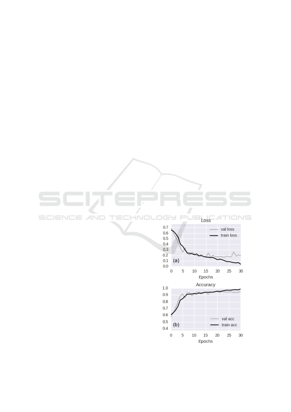
The CNN was trained for 30 epochs on our col-

orectal cancer training dataset, which lasted 8 hours

on Linux Inﬁniband-QDR MIMD Distributed Shared-

Memory Cluster provided with single GPU (NVIDIA

Tesla K40 - 12 GB - 2880 CUDA cores). Figure 4

shows the loss (a) and accuracy (b) curves on both the

training and validation datasets.

From the graphs of Figure 4 we can derive the fol-

lowing observations:

(i) The model seems to converge quite quickly. In-

deed, while training accuracy is still increasing,

the value of validation accuracy saturates within

15 epochs.

(ii) The decay speed of the validation loss curve in-

dicates that the learning rate is appropriate.

(iii) The similarity of validation and training accura-

cies reasonably rules out overﬁtting.

2.3 Transfer Learning From

Pre-trained CNN

A CNN is a cascade of trainable ﬁlter banks, where

the ﬁrst blocks of ﬁlters are devoted to the detection

of low-level features (i.e. edges or simple shapes),

and the following ones are activated by high-level se-

mantic aggregations of the previous patterns. While

the top-most blocks are generally tailored to a speciﬁc

classiﬁcation task, the lower-level features are ideally

generalisable to a large number of applications. This

concept, that is at the basis of all the transfer learning

techniques using CNNs as feature generators, lever-

age on the assumption that the network had ﬁrst been

trained on a very large set of examples, with signiﬁ-

cant variability of image characteristics.

In our work, we performed experiments using a

pre-trained CNN model with the same architecture

and building blocks of the one used for full train-

ing on colorectal cancer images (VGG16, shown in

Figure 2). The model was pre-trained on the Ima-

geNet dataset, from the Large Scale Visual Recog-

nition Challenge 2012 (ILSVRC-2012). The Ima-

Figure 4: Training vs validation loss per epoch (a) and train-

ing vs validation accuracy per epoch (b).

Colorectal Cancer Classiﬁcation using Deep Convolutional Networks - An Experimental Study

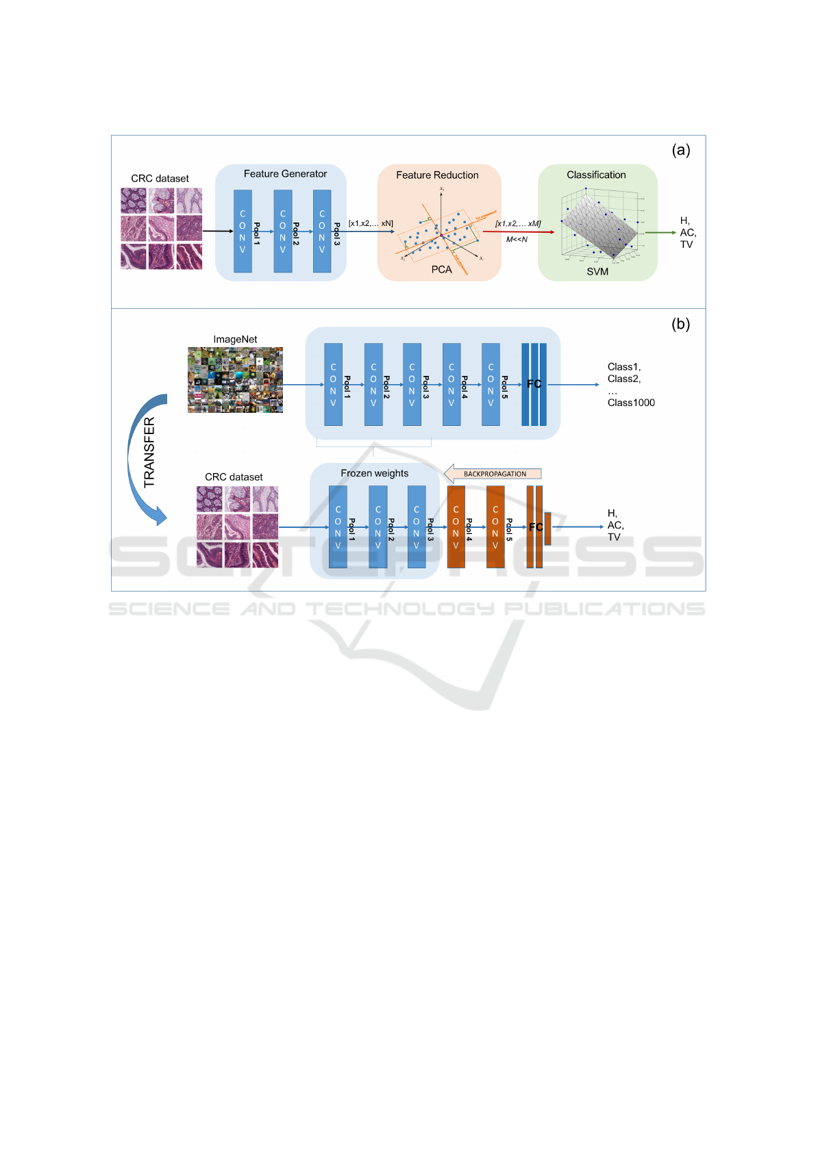
Figure 5: Transfer learning approaches. (a) Pre-trained CNN as a ﬁxed feature generator. (b) Fine tuning of pre-trained CNN.

geNet dataset contains 1.2 million photographs de-

picting 1000 different categories of natural objects.

Hence, the content and characteristics of the training

images are completely different from our speciﬁc tar-

get.

To apply the pre-trained CNN to our histology

classiﬁcation task, we implemented and compared

two different transfer learning approaches, whose

main steps are represented in Figure 5 (a) and (b), re-

spectively:

(i) CNN as a ﬁxed feature generator. The his-

tological images are given as input to the pre-

trained CNN for inference. The features ex-

tracted by the convolutional blocks are then fed

into a separate machine learning framework,

consisting of a feature reduction stage and a su-

pervised classiﬁer.

(ii) Fine-tuning the CNN. The CNN model is re-

trained on our training set of histological im-

ages, keeping all the parameters of the low-level

blocks ﬁxed to their initial value. Hence, only

the weights of the top-most layers are ﬁne-tuned

for colorectal cancer classiﬁcation.

As a preliminary step to both the two approaches,

we analysed the discriminative capabilities of the fea-

tures generated by all the major blocks of the pre-

trained CNN. More speciﬁcally, we randomly se-

lected a small subset of the training images (i.e. 1500

patches, 500 per class) and we fed these images into

the pre-trained CNN. The output of each successive

macro-block of the CNN was then analysed, to assess

the degree of separation of samples belonging to the

three different classes. As a trade-off between thor-

oughness and computational burden of the investiga-

tion, we analysed the intermediate output of the CNN

only at the end of the pooling layers (i.e. POOL1 to

5, in Figure 2). Indeed, as the pooling layers perform

a feature reduction on the output of the convolutional

ﬁlters, they are expected to produce a non-redundant

set of image features compared to CONV layers.

The degree of class separation was assessed by

means of t-Distributed Stochastic Neighbour Embed-

ding (t-SNE) (Maaten and Hinton, 2008), a non-linear

dimensionality reduction algorithm that is used for

BIOIMAGING 2018 - 5th International Conference on Bioimaging

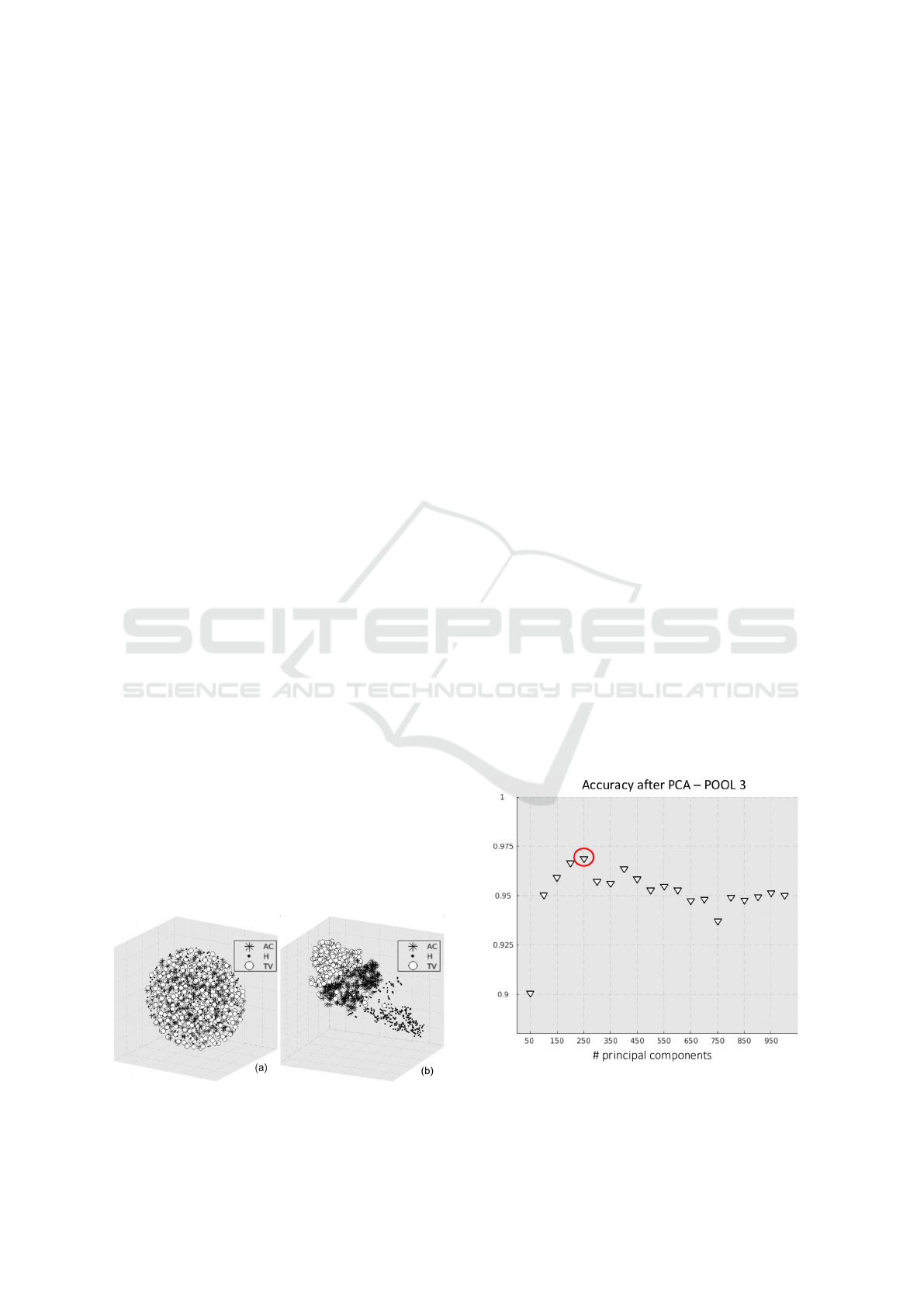
the visualisation of high-dimensional datasets in a re-

duced 3-dimensional space. More speciﬁcally, t-SNE

models each high-dimensional object (in our case, the

feature vector obtained at the output of a POOL layer)

by means of or three-dimensional point in a cartesian

space, so that similar feature vectors are represented

by nearby points and dissimilar vectors by distant

points. This allows to qualitatively assess the class

separability in the original feature space, and hence to

establish the POOL block that ensures the best class

separability (see examples in Figure 6).

The outcome of t-SNE was conﬁrmed by further

quantitative experiments, based on assessing the clas-

siﬁcation performance of a separate classiﬁer trained

on different POOL blocks. In all such experiments,

POOL3 outperformed all the other blocks.

2.3.1 Pre-trained CNN as A Fixed Feature

Generator

As ﬁrst transfer learning methodology, the output of

the most discriminative POOL layer of the pre-trained

CNN (in our case POOL3) was used to generate

a feature vector for colorectal cancer classiﬁcation.

The feature vector was fed into the machine learning

framework represented by Figure 5-(a), consisting in

a feature reduction and a classiﬁcation step.

(i) Feature reduction. Principal Component Anal-

ysis (PCA) was applied to reduce the dimen-

sionality of the input data and prevent overﬁt-

ting. PCA performs an orthogonal transforma-

tion of the original features into the so-called

principal components, a new group of values

which are linear combinations of the original

characteristics. As PCA works towards the min-

imisation of the correlation between the fea-

tures, the new data representation is expected to

best summarise those features which are most

representative for the classes of interest. In our

work, the optimal number of principal compo-

nents was empirically determined by means of

a sequential forward procedure. The mean clas-

Figure 6: t-SNE visualisation of the output of POOL2 (a)

and POOL3 (b).

siﬁcation accuracy obtained on the training set

was computed at increasing number of principal

components, with a step of 50. To limit the com-

putational cost of the procedure, we selected the

minimum number of principal components af-

ter which the classiﬁcation accuracy had started

decreasing, that was equal to 250 (see Figure 7).

(ii) Classiﬁcation. The ﬁnal classiﬁcation into

three categories (H, AC, TV) was performed by

a Support Vector Machine (SVM) with a Gaus-

sian radial basis function kernel. The hyper-

parameters of the kernel were set by means of a

Bayesian Optimisation (BO) algorithm (Hastie

et al., 2009), implementing a 10-fold cross-

validation procedure on the training images. BO

was found to provide much better and faster re-

sults compared to classic methods based on grid

search or heuristic techniques.

2.3.2 Fine-tuning of Pre-trained CNN

As a second transfer learning methodology, we tried

to adapt the pre-trained VGG16 net to our speciﬁc

classiﬁcation task. For this purpose, we ﬁrst ini-

tialised all the weights of the network to the ones

determined on the ImageNet dataset, as represented

in Figure 5-(b). Then, we continued the backprop-

agation procedure on our CRC dataset, keeping the

weights of the ﬁrst blocks of the net frozen. More

speciﬁcally, we froze all the weights up-to the most

discriminative pooling layer (POOL3), as determined

by t-SNE in Section 2.3. The rationale of such strat-

egy is trying to maintain the low-level features de-

scribing the most generic and generalisable details

Figure 7: Sequential forward procedure to select the optimal

number of principal components for PCA.

Colorectal Cancer Classiﬁcation using Deep Convolutional Networks - An Experimental Study

(e.g. edges and simple shapes) as they were learnt

from the ImageNet. Hence, all the computational

power can be devoted to the training of the top-most

layers, which are expected to learn high-level task-

speciﬁc features for colorectal image classiﬁcation.

The training strategy was exactly the same that was

described in Section 2.2.

3 CLASSIFICATION ACCURACY

3.1 Performance Metrics

The classiﬁcation performance was assessed using the

dataset described in Section 2.1. As already pointed

out, the test dataset is completely independent from

the one used for training the network and optimising

the classiﬁcation parameters. The accuracy of the sys-

tem was assessed at two different levels of abstraction

(per patch and per patient, respectively). For this pur-

pose, we introduce two different performance metrics.

(i) Patch score: (S

), deﬁned as the fraction of

patches of the test set that were correctly clas-

siﬁed:

where N

is the number of correctly classiﬁed

patches and N the total number of patches in the

test set.

(ii) Patient score: (S

), deﬁned as the fraction of

patches of a single patient that were correctly

classiﬁed (i.e. per-patient patch score), aver-

aged over all the patients in the test set:

∑

(i)

where S

(i) is the patch score of the i − th pa-

tient and N

the total number of patients in the

test set.

3.2 Results and Discussion

In Table 2 we report both the patch and patient scores

obtained for the three classiﬁcation frameworks de-

scribed in Section 2. More speciﬁcally:

(i) full-train-CNN refers to the CNN fully trained

on CRC samples.

(ii) CNN+SVM: refers to the SVM, with pre-

trained CNN used as ﬁxed feature generator.

(iii) ﬁne-tune-CNN: refers to the pre-trained CNN

with ﬁne-tuning of the ﬁnal stages.

For the patient score, S

value is reported as

mean ± standard deviation. From the results of

Table 2 we can observe that all the proposed clas-

siﬁcation frameworks obtained accuracy (both patch

and patient-wise) above 90%. Hence, the promising

results obtained by CNNs in other contexts are con-

ﬁrmed even for the application targeted by our work.

On top of that, the accuracy computed over all the

patches of the test set (S

) is very similar to the one

computed patient per patient (S

), with a very small

standard deviation of the latter value. This suggests

that the classiﬁcation frameworks are all quite robust

and cope well with inter-patient variability, that is a

typical challenge of histopathological image analysis.

The same conclusions hold if we analyse the per-

class results, that are reported in the form of 3X3 con-

fusion matrices in Figure 8. In addition, from the

confusion matrices we can observe that the perfor-

mance of the classiﬁcation frameworks is fairly ho-

mogeneous for the three classes H, AC and TV.

Quite interestingly, both the methodologies based

on transfer learning overcome the accuracy obtained

by the CNN fully trained on colorectal samples by al-

most 7%. In particular, the approach that provided

the best accuracy values (both patch and patient-

wise) was the pre-trained CNN with ﬁne-tuning of the

blocks following POOL 3. This suggests the follow-

ing:

(i) Even though the full training seemed to con-

verge well and without overﬁtting on the train-

ing images (see Figure 4), the CNN would prob-

ably necessitate a much larger cohort of exam-

ples to learn features that are sufﬁciently general

to cope with the high variability of histopatho-

logical images. On the other hand, much larger

training datasets would make the learning pro-

cess prohibitive, especially in a clinical context.

(ii) In spite of the fact that the pre-training was

performed on a completely different dataset

(i.e. the ImageNet, which contains photographs

of every-day objects and natural scenes, and

not histological samples), the low-level features

learnt by the ﬁrst stages of a CNN can be suc-

cessfully generalised to the context of CRC im-

age classiﬁcation. Hence, CNNs are as a mat-

ter of fact capable of extracting usable seman-

tic knowledge from totally different domains.

This is very encouraging, as it partially avoids

Table 2: Patch and patient scores on the test set.

full-train-CNN 0.9037 0.9022 (± 0.0155)

CNN+SVM: 0.9646 0.9667 (± 0.0082)

ﬁne-tune-CNN 0.9682 0.9678 (± 0.00092)

BIOIMAGING 2018 - 5th International Conference on Bioimaging

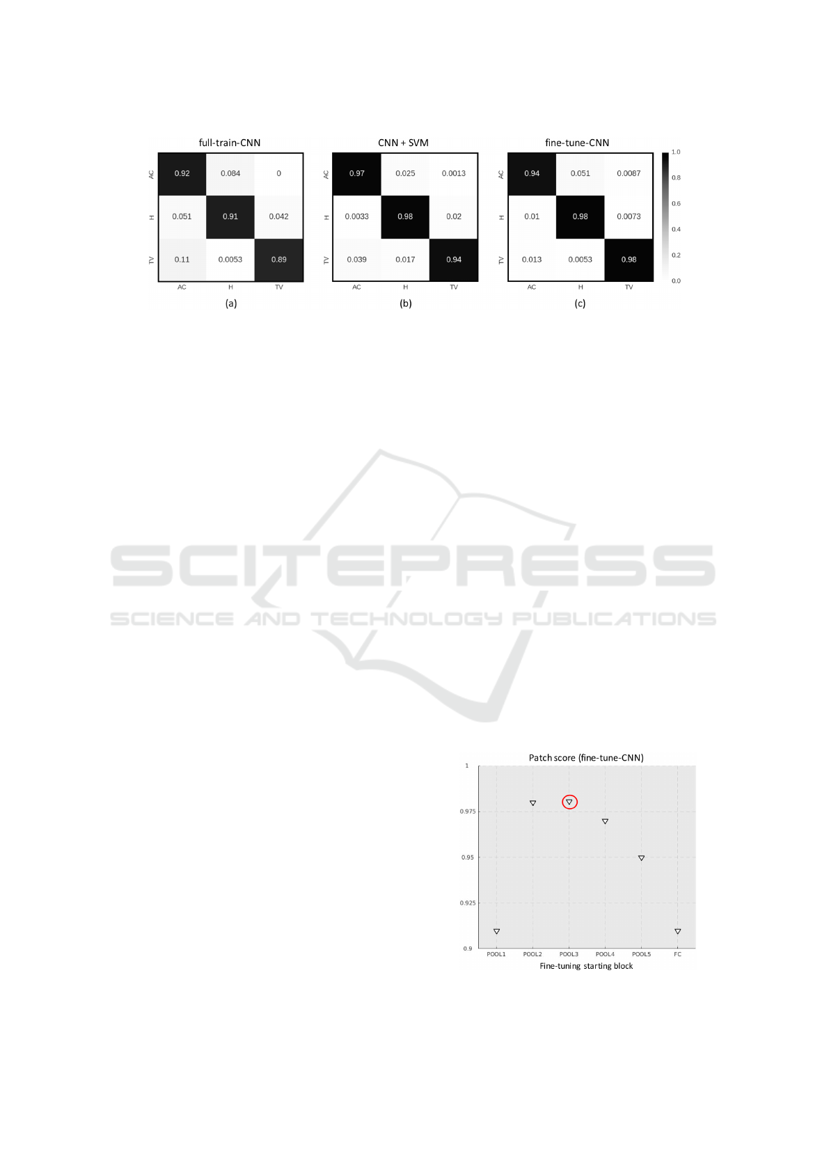
Figure 8: Patch-wise confusion matrices for (a) CNN fully trained on CRC samples, (b) SVM with pre-trained CNN as ﬁxed

features generator, (c) pre-trained CNN with ﬁne-tuning of the stages after POOL3 block.

the computational problems and overﬁtting risks

associated with full-training. Indeed, the ﬁne-

tuning of the pre-trained CNN took only two

hours against the eight taken by full-training, us-

ing the same hardware and learning paradigm.

To investigate further on the performance of the

ﬁne-tuned CNN, we run additional experiments by

changing the starting block for the backpropagation

algorithm. In Figure 9, we report the patch score ob-

tained on the test set, for different conﬁgurations of

the ﬁne-tuning. In the x-axis, POOL-i means that only

the weights after the i-th POOL block were learnt on

the CRC training set, while all the rest of the parame-

ters were frozen to the values learnt on the ImageNet.

Likewise, FC means that only the fully-connected

stage of the network was trained. The trend of the

patch score values shows that the maximum accuracy

is reached when the CNN is ﬁne-tuned after POOL3,

which conﬁrms the qualitative results of t-SNE. On

top of that, we can observe that fully-training the net-

work obtains more or less the same results than train-

ing only the last fully-connected stage. This further

conﬁrms that CNN can be successfully used to trans-

fer features learnt from the ImageNet.

4 CONCLUSIONS AND FUTURE

WORK

In this work we investigated the use of deep learning,

and more speciﬁcally of Convolutional Neural Net-

works, for the automated classiﬁcation of colorectal

histology samples into three main classes of interest:

healthy tissue, adenocarcinoma or tubulovillous ade-

noma.

For this purpose, we applied a CNN with VGG16

architecture, which we fully trained on a large dataset

of pre-annotated images of colorectal samples. This

solution provided satisfactory results when applied to

an independent test dataset, with classiﬁcation accu-

racy in the order of 90%.

Besides the traditional full training approach, we

investigated two types of transfer learning techniques:

(i) using the ﬁrst convolutional stages of a CNN pre-

trained on the ImageNet as a ﬁxed feature genera-

tor for a Support Vector Machine, with a preliminary

feature reduction step; (ii) using the colorectal train-

ing set to ﬁne-tune the last convolutional and fully-

connected stages of the pre-trained CNN.

In our experiments the transfer learning tech-

niques outperform the full training approach both in

terms of classiﬁcation accuracy (above 96%) as well

as in terms of training time. Hence, they demonstrate

that low-level features learnt by the CNN in a very dif-

ferent context (the ImageNet, in this case) can be suc-

cessfully transferred to the classiﬁcation of colorectal

images.

As a future work, we plan to extend the classiﬁ-

cation problem to more tissue categories (i.e. differ-

ent types of benign lesions, besides tubulovillous ade-

noma). In the long run, we plan to design a develop

a complete framework for the analysis of colorectal

WSIs based on CNNs.

Figure 9: Mean accuracy in relation to the ﬁrst block till

back-propagation is continued.

Colorectal Cancer Classiﬁcation using Deep Convolutional Networks - An Experimental Study

REFERENCES

A. Young, R. H. and Kerr, D. (2011). ABC of Colorectal

Cancer. Wiley-Blackwell, 2nd edition.

Chollet, F. et al. (2015). Keras.

https://github.com/fchollet/keras.

Di Cataldo, S. and Ficarra, E. (2017). Mining textu-

ral knowledge in biological images: Applications,

methods and trends. Computational and Structural

Biotechnology Journal, 15:56 – 67.

Hastie, T., Tibshirani, R., and Friedman, J. (2009).

Overview of supervised learning. In The elements of

statistical learning. Springer.

Janowczyk, A. and Madabhushi, A. (2016). Deep learn-

ing for digital pathology image analysis: A compre-

hensive tutorial with selected use cases. Journal of

Pathology Informatics, 7(1):29.

Korbar, B., Olofson, A. M., Miraﬂor, A. P., Nicka, C. M.,

Suriawinata, M. A., Torresani, L., Suriawinata, A. A.,

and Hassanpour, S. (2017). Deep learning for clas-

siﬁcation of colorectal polyps on whole-slide images.

Journal of Pathology Informatics, 8:30.

Maaten, L. v. d. and Hinton, G. (2008). Visualizing data

using t-sne. Journal of Machine Learning Research,

9(Nov):2579–2605.

Marley, A. R. and Nan, H. (2016). Epidemiology of col-

orectal cancer. International Journal of Molecular

Epidemiology and Genetics, 7(3):105–114.

Qian, N. (1999). On the momentum term in gradi-

ent descent learning algorithms. Neural networks,

12(1):145–151.

Simonyan, K. and Zisserman, A. (2014). Very deep con-

volutional networks for large-scale image recognition.

arXiv preprint arXiv:1409.1556.

Weiss, K., Khoshgoftaar, T. M., and Wang, D. (2016). A

survey of transfer learning. Journal of Big Data,

3(1):9.

Yao, Y., Rosasco, L., and Caponnetto, A. (2007). On early

stopping in gradient descent learning. Constructive

Approximation, 26(2):289–315.

BIOIMAGING 2018 - 5th International Conference on Bioimaging