Evaluation of Transfer Learning Scenarios

in Plankton Image Classiﬁcation

Francisco Caio Maia Rodrigues

, Nina S. T. Hirata

, Antonio A. Abello

, Leandro T. De La Cruz

Rubens M. Lopes

and R. Hirata Jr.

Institute of Mathematics and Statistics, University of S

ao Paulo, Rua do Mat

ao 1010, S

ao Paulo - SP, Brazil

Institute of Oceanography, University of S

ao Paulo, Prac¸a do Oceanogr

aﬁco 191, S

ao Paulo - SP, Brazil

Keywords:

Transfer Learning, Plankton Classiﬁcation, CNN, SVM, Alexnet, ImageNet.

Abstract:

Automated in situ plankton image classiﬁcation is a challenging task. To take advantage of recent progress

in machine learning techniques, a large amount of labeled data is necessary. However, beyond being time

consuming, labeling is a task that may require frequent redoing due to variations in plankton population

as well as image characteristics. Transfer learning, which is a machine learning technique concerned with

transferring knowledge obtained in some data domain to a second distinct data domain, appears as a potential

approach to be employed in this scenario. We use convolutional neural networks, trained on publicly available

distinct datasets, to extract features from our plankton image data and then train SVM classiﬁers to perform

the classiﬁcation. Results show evidences that indicate the effectiveness of transfer learning in real plankton

image classiﬁcation situations.

1 INTRODUCTION

Plankton communities form the basis of aquatic food

webs and exert a major inﬂuence on material cycles

relevant to global climate change, such as carbon di-

oxide and methane. Therefore, it is essential to under-

stand the spatial distribution and temporal variability

of planktonic organisms in the ocean. Plankton col-

lection and analysis has been traditionally carried out

by net tows and subsequent microscopic inspection

of preserved samples. Such approach has led to a

signiﬁcant increase in the knowledge about taxono-

mic composition and distribution of several plankton

groups, but ﬁne-scale sampling is usually not feasible

with nets and many fragile organisms are destroyed

by collision with the net mesh or disintegrate in ﬁxa-

tives.

Recent advances in digital image acquisition and

Machine Learning (ML) techniques have stimulated

the application of in situ imaging to generate highly

resolved vertical proﬁles of plankton composition and

abundance (counts per volume). While high-quality

image acquisition technologies represent the ﬁrst step

in such task, new approaches in ML techniques are

in the core of our increasing capability to deal with

the complex and highly variable geometry of plankton

organisms.

Convolutional Neural Networks (CNN) have

emerged as a powerful technique for image classiﬁca-

tion and its variants are being successfully employed

on a variety of classiﬁcation tasks. The characteristic

of being data-driven, not requiring speciﬁcally desig-

ned features, make them a suitable model to cope with

the high variability of plankton species distribution in

space and time. However, the training success of such

models depends not only on experimentation and ad-

justment of parameter values but on the availability of

large amount of training data. This is a critical point

in supervised learning tasks such as classiﬁcation.

There have been some efforts to make available

labeled plankton image datasets. The International

Council for the Exploration of the Sea (ICES)

initiative, http://www.ices.dk/marine-data/dataset-

collections/Pages/Plankton.aspx and the Kaggle’s

National DataScience Bowl (NDSB) competition, via

the In Situ Icthyoplankton Imaging System (ISIIS),

https://www.kaggle.com/c/datasciencebowl, are a

few of the examples. These datasets may differ lar-

gely with respect to plankton composition and image

quality. Diversity may originate from differences in

locations (geographical and along the water column),

in imaging technologies which may target plankton

of different size ranges, or even in the goals of the

research project. Due to those differences, available

Rodrigues, F., Hirata, N., Abello, A., Cruz, L., Lopes, R. and Jr., R.

Evaluation of Transfer Learning Scenarios in Plankton Image Classiﬁcation.

DOI: 10.5220/0006626703590366

In Proceedings of the 13th International Joint Conference on Computer Vision, Imaging and Computer Graphics Theory and Applications (VISIGRAPP 2018) - Volume 5: VISAPP, pages

359-366

ISBN: 978-989-758-290-5

359

datasets may not be directly useful to the application

context of a given research program. At the same

time, labeling a large amount of data each time a set

of observations with new characteristics is available

is unfeasible.

One approach to deal with these types of situati-

ons is transfer learning (TL) (Pan and Yang, 2010).

In ML

, TL expresses the concept of using or adap-

ting a model induced in a speciﬁc context to another

context. For instance, using or adapting a model le-

arned using a plankton dataset from Atlantic ocean to

classify another one from the Paciﬁc ocean.

In this work we investigate TL applied to plankton

classiﬁcation. Our goal is to develop an algorithm to

classify samples in our in-house dataset. Since we fo-

resee different deployment scenarios in the future, we

would like to have a data-driven classiﬁcation appro-

ach. Therefore, CNNs appear as an interesting option

except by the fact that the small size of our dataset

makes training such a model from scratch an unfea-

sible task and thus we resort to adapt pre-trained mo-

dels as feature extractors. Taking advantage of the

fact that there exists a public available massive data-

set of plankton images used in previously mentioned

Kaggle’s NDSB competition, our approach is to train

a CNN, speciﬁcally the one proposed by the winning

team, using this dataset to extract meaningful featu-

res from our smaller in-house built dataset. Although

there are differences in the datasets with respect to

the classes of plankton species they include, either

because a particular species or class in one of the da-

tasets is not in the other , it is reasonable to expect

that they could be efﬁciently classiﬁed by the same

set of features. To further investigate the quality of

the features obtained from this process, we also em-

ploy a different CNN trained on this same dataset and

on ImageNet (Russakovsky et al., 2015), which con-

tains images from a completely distinct domain. By

using CNNs and external domain source datasets, we

would like to understand how transfer learning per-

forms and whether an external dataset will help or not

the classiﬁcation of our data.

Plankton image classiﬁcation using CNNs star-

ted to be considered only recently (Al-Barazanchi

et al., 2015; Dai et al., 2016; Py et al., 2016) and, in

particular, transfer learning of features computed by

CNNs (Orenstein and Beijbom, 2017) has not been

explored much yet in this context. The present con-

tribution aims to deepen our understanding of transfer

learning in planktonic data.

The remaining of the text is organized as follows.

In Section 2 we brieﬂy recall the transfer learning for-

The concept is used in Psychology and Education Re-

search, as well.

mulation and outline the methods to be used in our ex-

periments. In Section 3 we describe the datasets and

CNN models to be used. Then, in Section 4 we detail

the experiments and discuss the results. We present

the conclusions of this work in Section 5.

2 METHOD OVERVIEW

Given an input space of observations, denoted as X ,

and a set of class labels, denoted as Y , classiﬁcation

can be modeled as the problem of predicting a class

label y for each instance x in X . Assuming there is

a joint probability distribution p on X ×Y , the mini-

mum error classiﬁcation can be determined from the

conditional probabilities p(y|x). Discriminative ap-

proaches in supervised machine learning often tries,

for each input x, to approximate their outputs to the

probabilities p(y|x).

In classiﬁcation, X deﬁnes a domain and Y deﬁnes

a task. Elements in X usually consist of convenient

encodings of objects to be classiﬁed and set Y consists

of the corresponding class labels for each element in

X . For instance, X could represent the feature vec-

tors extracted from plankton images and set Y could

be a set of numbers representing the taxonomy of the

different species of plankton.

In many situations, there is no sufﬁcient amount

of labeled data to train a classiﬁer in a given target

domain. Among the approaches used to handle this

type of situation, there is for instance data augmenta-

tion (Simard et al., 2003), transfer learning (Pan and

Yang, 2010), and bootstrap methods (Hastie et al.,

2009). Transfer learning refers to using knowledge

obtained from a distinct domain data, and possibly

distinct task, to learn the conditional probability dis-

tribution of the target domain.

Representations learned by CNNs are reported to

be very useful for the classiﬁcation of data, even

in distinct domains (Bengio, 2012; Yosinski et al.,

2014). The usual approach to exploit this is to select

an intermediate layer as a target layer, freeze it and

its preceding layers and adjust the subsequent layers.

The earlier the layer chosen, the more general and the-

refore, more transferable the representation is (Yosin-

ski et al., 2014), but also the more data is necessary

to adjust it, since it has a higher dimension. The ad-

justment of subsequent layers may be done via ﬁne-

tuning, continuing training with new samples, or by

training an entirely new classiﬁer from scratch using

the output of the intermediate target layer as features,

which is called (deep) feature extraction. In this work

we chose the latter option, using pre-trained CNNs as

feature extractors.

VISAPP 2018 - International Conference on Computer Vision Theory and Applications

360

The experiments have been designed to answer the

following questions:

• how DeepSea trained on ISIIS (NDSB competi-

tion) – DeepSea(ISIIS) – will perform on our in-

house dataset (LAPSDS)?

• how classiﬁers using features extracted from

DeepSea(ISIIS) will perform on LAPSDS?

• how classiﬁers using features extracted from

AlexNet trained on ISIIS – AlexNet(ISIIS) – will

perform on LAPSDS?

• how classiﬁers using features extracted

from AlexNet trained on ImageNet – Alex-

Net(ImageNet) – will perform on LAPSDS?

In addition to these TL scenarios, we also con-

sider the traditional feature extraction approach that

will serve as a baseline. Diagram in Fig. 1 summari-

zes the scenarios to be evaluated. Four sets of features

are extracted from LAPSDS and they are used to train

SVM classiﬁers as detailed ahead in Section 4.

ISIIS

train DeepSea

DeepSea(ISIIS)

apply

CNN feature

extraction

train AlexNet

AlexNet(ISIIS)

apply

CNN feature

extraction

ImageNet

train AlexNet

AlexNet(ImageNet)

apply

CNN feature

extraction

LAPSDS

shape feature

extraction

Figure 1: Deep feature extraction scenarios considered

here. ISIIS ImageNet and LAPSDS denote image datasets,

gray shaded nodes indicate the pre-trained CNNs, and CNN

feature extraction consists of extracting the values from a

speciﬁc layer of a CNN, after a forward pass of samples in

LAPSDS.

3 DATASETS AND CNN MODELS

In this section, we describe the datasets and the two

chosen CNN models used in the experiments.

3.1 Datasets

3.1.1 LAPS Dataset (LAPSDS)

In situ plankton images have been acquired with a

submersible instrument developed at our lab LAPS-

IOUSP

. The instrument has been vertically deployed

between surface and 30m depth off the lab base

and

gray-scale images were acquired at approximately 15

frames per second, with dimensions of 2448 × 2050

pixels and resolution of ∼5µm. Image stacks belon-

ging to the same vertical proﬁle were converted into

video ﬁles to mitigate data storage and management.

A total of 230,000 Regions of Interest (ROI) were ex-

tracted from 16 selected videos and 5175 ROIs were

used in the creation of in-house dataset. A labeling

process was carried by plankton experts belonging to

the same lab.

LAPSDS is composed of 20 classes containing at

least 100 samples each, and as expected, the number

of images varies from class to class. Table 1 shows the

class distribution of the dataset, as well as the name

and the identiﬁer number of each class. Instances of

some of the classes are shown in Fig. 2.

Table 1: Histogram of classes of the LAPSDS.

ID H classes Size ID H classes Size

0 appendicularia 216 10 detritus uf 286

shape s stick bw

1 appendicularia 114 11 dinoﬂagellates 242

curve tripus 2

2 cladocera 435 12 dinoﬂagellates 316

tripus

3 copepod calanoid 315 13 nauplii 465

4 copepod cyclopoida 106 14 phytoplankton 0 259

5 copepod 163 15 phytoplankton 1 127

poecilostomatoida

6 detritus df bk 288 16 phytoplankton 5 159

7 detritus uf dot bk 344 17 chaetocero 546

8 detritus uf dot bw 274 18 diatoms 120

coscinodiscus

9 detritus uf stick bk 152 19 shadow 249

In-situ images are prone to natural variability in

illumination, turbulent ﬂow and turbidity, among ot-

her factors, which may compromise image quality be-

cause ROIs from different videos may have different

background intensities (see Fig.2). Thus, for conve-

nience, the background of the ROIs have been re-

moved using a technique of background subtraction

adapted to deal with illumination changes (Jacques

et al., 2006). An example is shown in Fig. 3.

Laboratory of Plankton Systems, Oceanographic Insti-

tute, University of S

ao Paulo, Brazil

(lat:-23.499913, long:-45.119381)

Evaluation of Transfer Learning Scenarios in Plankton Image Classiﬁcation

361

Figure 2: Image sample from LAPSDS. Number on the ROI

indicates the class that they belong to.

(a) (b)

Figure 3: Background removal example: (a) Original

image, labeled as “appendicularia shape s” and (b) result

of the background removal of image in (a).

3.1.2 Kaggle’s National Data Science Bowl

The National Data Science Bowl (NDSB) was a com-

petition hosted by Kaggle in a collaboration with Ore-

gon State University’s Hatﬁeld Marine Science Cen-

ter. Several research teams competed to develop and

train supervised classiﬁers, given a dataset provided

by the Hatﬁeld Marine Science Center(Cowen et al.,

2015).

According to the competition organizers, the ima-

ges were collected in the Straits of Florida using

an underwater imaging system called ISIIS (In Situ

Ichthyoplankton Imaging System). It captured high-

resolution continuous images that were parsed in

2048x2048 pixel frames. The resulting frames were

thresholded and segmented. Finally, regions of inte-

rest were extracted and became the images that com-

prise the dataset after being annotated by the Marine

Science Center’s personnel.

The dataset was divided by taxonomy, behavior

and shape into 121 classes. Each class contained

between 9 and 1979 individual examples, totalizing

30,336 images.

3.1.3 ImageNet

ImageNet is a dataset that became one of the ben-

chmarks for object classiﬁcation and detection. It

Figure 4: Assorted plankton from the ISIIS dataset. Each

sample is from a different class. Note the absence of back-

ground.

is comprised of over 14 million images divided into

1000 classes hierarchically subdivided (Russakovsky

et al., 2015). The classes subjects range from human

persons to animals and fungi to everyday objects, con-

stituting a very general dataset. Since 2010 a competi-

tion including diverse tasks such as classiﬁcation and

detection on pictures or video on this dataset is held

each year.

3.2 CNN MODELS

The two network architectures used in this work are

from winning teams in computer vision competitions.

They are the AlexNet (Krizhevsky et al., ), from the

2012 ImageNet Large Scale Visual Recognition Com-

petition (ILSVRC), and a model from the ”Deep Sea”

team, that won Kaggle’s ISIIS in 2014.

3.2.1 AlexNet

AlexNet is a Convolutional Neural Network model

that was introduced in the ILSVRC held in 2012. Un-

der the team name of ”SuperVision”, it won both the

classiﬁcation and localization tasks by a large mar-

gin

, being the ﬁrst case of success in applying this

kind of model in the competition and establishing a

strong trend of its use in the next years.

This model introduced and popularized a lot of

novelty features for improving training time, perfor-

mance and reducing overﬁtting including, but not li-

mited to: ReLU , Dropout and Local Response Nor-

malization. We refer to the original paper for a more

http://image-net.org/challenges/LSVRC/2012/results

VISAPP 2018 - International Conference on Computer Vision Theory and Applications

362

(a) AlexNet

(b) DeepSea’s convroll4 network

Figure 5: Neural Networks architectures used in the experiments. Although DeepSea’s model is much deeper than AlexNet,

it has less parameters (i.e. ﬁlters in Convolutional layers and units in Fully Connected layers) to ﬁt during the training. The

dashed boxes indicate which layer was used in the transfer learning experiments.

detailed explanation of these innovations and their im-

pact (Krizhevsky et al., ) (see Fig. 5(a) for a represen-

ting diagram of the CNN).

We did not explicitly train AlexNet model in the

ImageNet dataset, but used instead a pre-trained mo-

del with available weights online

. In order to feed

our images to this model, a couple minor modiﬁ-

cations were required, such as converting our one-

channel grayscale images to three-channels RGB and

resizing, via a wrap padding tactic, to match the ex-

pected input.

AlexNet implementation that was trained on ISIIS

dataset was heavily based on DeepSea’s model, fol-

lowing exactly the same training procedure for both

networks (i.e. data preprocessing and data augmen-

tation). Thus, this network’s input expects grayscale

images with size 95x95 and its ﬁnal layer contains

121 units.

3.2.2 Deep Sea’s Model

Deep Sea was the winning team of the Kaggle ISIIS.

They used an approach of ensembling multiple deep

learning models with minor differences to improve

generalization. We used the most simple model avai-

lable, consisting solely of a CNN, which here we call

DeepSea.

The main innovation brought by the team was a

couple of layers designed to increase the network ro-

bustness to cyclic variation (Dieleman et al., 2016). In

the ”cyclic slice” layer the input is rotated four times

and processed separately by the network from that

point onward. Then, in the ”cyclic roll” layer, the fea-

ture maps from the four paths are permuted and inter-

changed. Eventually, in the ”cyclic pooling” layer the

four network paths are merged again into a single one.

We again refer to the paper on this architecture for

a more detailed explanation (Dieleman et al., 2016)

(see Fig. 5(b) for a representing diagram of the CNN).

https://github.com/BVLC/caffe/tree/master/models/bv

lc alexnet

4 EXPERIMENTS AND

DISCUSSION

Experiments followed the outline presented in

Section 2. Given a pre-trained CNN, the steps to be

executed consist of feature extraction, classiﬁer trai-

ning, and classiﬁer performance evaluation. We des-

cribe these steps in the subsequent sections and at the

end we present some discussions.

4.1 Feature Extraction

4.1.1 Deep Features

From DeepSea(ISIIS). The features were extracted

from the output of the last Cyclic Pooling Layer, as

shown in Figure 5(b) highlighted by enclosing das-

hed lines, resulting in 256 features per images. These

features correspond to F1 in the diagram of Fig. 1.

In a Cyclic Pooling Layer the effect of rotations intro-

duced by previous Cyclic Slice and Cyclic Roll layers

are undone, hence capturing the output from this layer

is the most appropriate choice since we can leverage

on the learned invariances.

From AlexNet(ISIIS) and AlexNet(ImageNet).

From the two pre-trained AlexNet, AlexNet(ISIIS)

and AlexNet(ImageNet), features were extracted from

the ﬁrst Fully Connected layer, as shown in Fi-

gure 5(a) highlighted by enclosing dashed lines, re-

sulting in 4096 features per image. These features

correspond to F2 and F3, respectively, in the diagram

of Fig. 1.

4.1.2 Shape Features

We extracted 74 features commonly used in traditio-

nal shape recognition procedures. They are divided

into the following three categories:

Evaluation of Transfer Learning Scenarios in Plankton Image Classiﬁcation

363

• 54 shape features (area, perimeter, solidity, con-

vexity, etc). Most of the feature descriptors are

implemented in the OpenCV library and they are

usually presented in automatic plankton classiﬁ-

cation works that use shape features (Blaschko

et al., 2005).

• 10 from Local Binary Patterns (LBP) histo-

grams (Ojala et al., 2000) extracted using a 3 × 3

window.

• 10 from Haralick descriptors, extracted from the

co-occurrence matrix (Haralick et al., 1973).

Shape and LBP features are extracted from the

images segmented using Otsu’s threshold (Otsu,

1979). Haralick’s descriptors are extracted from gray-

level images. These features correspond to F4 in the

diagram of Fig. 1.

4.2 Classiﬁer Training and Evaluation

To train and evaluate the SVM classiﬁers with respect

to each of the four feature sets, we performed a 9:1

train-test split that preserved class proportions. This

split resulted in a training set of 4658 and a test set of

517 samples.

Before training, a data normalization to convert

all feature values to the [0.0, 1.0] range was applied

to each individual feature of the four feature sets. The

normalization parameters were inferred using the trai-

ning samples in order to not add bias to the classiﬁer.

Test samples were then transformed by those same pa-

rameters.

Sklearn’s (Pedregosa et al., 2011) grid search with

cross-validation was employed to explore the space of

possible parameters for SVM, namely the kernel type,

value of C and, if a RBF kernel was used, γ values. In

this work, we considered linear and RBF kernels, C ∈

{1, 10, 100, 200} and γ ∈ {0.01, 0.001, 0.0001,

n f

where n f is the number of features, this is a common

well-known heuristics. The best parameters found for

each feature set are displayed on Table 2. The same

table also shows the overall accuracies computed on

test set.

Table 2: Table summarizing the results obtained from dif-

ferent transfer learning scenarios. The value of 0.0002 for

γ was selected because of the

n f

option. Accuracy refers to

the test set.

Feature extractor

SVM parameters

Acc.

kernel C γ

DeepSea(ISIIS) rbf 100 0.01 84%

AlexNet(NSDB) rbf 10 0.01 81%

AlexNet(ImageNet) rbf 100 0.0002 80%

Shape Features linear 100 - 72%

4.3 Discussions

Global accuracy alone, specially in cases as ours,

where the methods present similar performance, is not

much informative. To better understand the results,

we plotted a confusion matrix (Fig. 6) for each fea-

ture set.

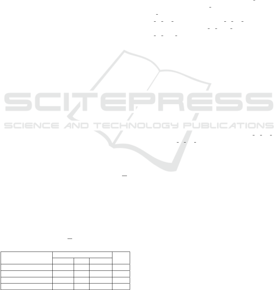
As it can be seen, the ﬁrst plot corresponding to

DeepSea(ISIIS), the one that achieved the best per-

formance, has a darker diagonal compared to the ot-

her plots. Confusion is larger in the last plot, the

one that is based on shape features. In general,

there is confusion between class 3 (copepod calanoid)

and classes 4 (copepod cyclopoida) and 5 (cope-

pod poecilostomatoida), between classes 7 (detri-

tus uf dot bk) and 8 (detritus uf dot bw), and be-

ween classes 9 (detritus uf skick bk) and 10 (detri-

tus uf stick bw). Figure 7(a) presents some examples

of copepods subtypes that can confuse the classiﬁers.

The ﬁgure is organized in three columns, one for each

copepod subtype: column 1 shows four examples of

calanoids, column 2 shows three examples of cyclo-

poida, column 3 shows four examples of poecilosto-

matoids. Each image is labeled with zero to four co-

lored squares that represent the success of the corre-

sponding classiﬁer in classifying correctly that image.

As one can see, the plankton belonging to these clas-

ses are similar in several aspects and it is not difﬁcult

to understand why these classes cause confounding

errors. A similar scenario has been found for detrital

particles. Figure 7(b) presents a similar set of images

of examples of detritus subtypes (detritus uf dot bk

and detritus uf dot bw) that can confuse the classi-

ﬁers.

Another view of the results is shown in Fig. 8. We

present a bar chart displaying the accuracy of each

classiﬁer per class. Classes 2, 11, 12, 13 and 18 were

well classiﬁed by all the four classiﬁers and therefore

they could be considered as the easy classes. On the

other hand, classes 4 and 9 are those where most clas-

siﬁers did poorly, and thus they are the hardest ones.

Classes 0 and 1 are those with the largest variation

between the best and worst performing classiﬁers.

Hand designed features performed clearly worse

than any of the CNN extracted ones. Although no

careful feature selection was performed, it is also true

that no careful deep feature extraction was performed.

Thus, in a situation where a quick solution is required,

making use of a pre-trained CNN could be more ef-

fective than using a large set of hand designed feature

extractors.

VISAPP 2018 - International Conference on Computer Vision Theory and Applications

364

Figure 6: Confusion Matrices.

(a) Cyclopoida, Calanoid, Poecilostomatoida (b) uf dot bk, uf dot bw

Figure 7: Two sets of plankton images from confounding classes.

Figure 8: Class accuracy histogram.

5 CONCLUSIONS

We have presented an evaluation of transfer learning

scenarios in the context of plankton image classiﬁca-

tion. We have used CNNs pre-trained on external da-

tasets as feature extractors from our in-house dataset

images. In particular, we have considered two very

distinct external datasets, one of plankton images (and

thus similar to our data) and another of natural images

(ImageNet), and the corresponding “winning” CNN

architectures. Transfer learning experiments showed

that the architecture developed for plankton images

(DeepSea) performed better than the architecture de-

veloped for natural image classiﬁcation (AlexNet),

even when both were trained with the same plankton

image dataset. We also observed that AlexNet trai-

ned on natural images performed almost as well as the

same network trained on plankton images. These two

observations indicate that in transfer learning using

CNNs, the architecture may play an important role,

even larger than the dataset per se. To complement

these observations, it would be interesting to train

Evaluation of Transfer Learning Scenarios in Plankton Image Classiﬁcation

365

DeepSea with ImageNet and evaluate how well it will

perform on our data.

Overall, our conclusion is that transfer learning

using CNNs as feature extractors might be an ef-

fective approach to cope with large scale and high

variability of plankton images. However the optimal

choice of external datasets and network architectures

are still not well understood and should be further in-

vestigated in order to push up the accuracy. For fu-

ture works we plan to experiment with ensemble of

classiﬁers, as already done by DeepSea team and also

do data augmentation by blurring the well focused

images in a way that resembles the bad focused ones

(classiﬁers usually do not perform well when classi-

fying images with this kind of problem).

ACKNOWLEDGEMENTS

Funding was provided by CAPES (CIMAR

2001/2014), CNPq (565062/2010-7, 311936/2013-0,

400221/2014-4 and 446709/2014-0) and FAPESP

(13/17633-6, 2015/01587-0).

REFERENCES

Al-Barazanchi, H. A., Verma, A., and Wang, S. (2015).

Performance Evaluation of Hybrid CNN for SIPPER

Plankton Image Class. In 2015 Third Int. Conf. on

Image Inf. Processing (ICIIP), pages 551–556.

Bengio, Y. (2012). Deep Learning of Repr. for Unsupervi-

sed and Transfer Learning. In Proc. of ICML Work. on

Unsuperv. and Transf. Learning, pages 17–36.

Blaschko, M. B., Holness, G., Mattar, M. A., Lisin, D.,

Utgoff, P. E., Hanson, A. R., Schultz, H., and Rise-

man, E. M. (2005). Automatic in situ identiﬁcation of

plankton. In App. of Computer Vision. Seventh IEEE

Workshops on WACV/MOTIONS’05, volume 1, pages

79–86. IEEE.

Cowen, K., R., Sponaugle, S., Robinson, K., and Luo, J.

(2015). PlanktonSet 1.0: Plankton imagery data col-

lected from F.G. Walton Smith in Straits of Florida

from 2014-06-03 to 2014-06-06 and used in the 2015

National Data Science Bowl.

Dai, J., Wang, R., Zheng, H., Ji, G., and Qiao, X. (2016).

ZooplanktoNet: Deep Conv. Network for Zooplank-

ton Classiﬁcation. In OCEANS 2016 - Shanghai, pa-

ges 1–6.

Dieleman, S., Fauw, J. D., and Kavukcuoglu, K. (2016). Ex-

ploiting Cyclic Symmetry in Conv. Neural Networks.

CoRR, abs/1602.02660.

Haralick, R. M., Shanmugam, K., et al. (1973). Textural

features for image classiﬁcation. IEEE Transactions

on systems, man, and cybernetics, 3(6):610–621.

Hastie, T., Tibshirani, R., and Friedman, J. (2009). The Ele-

ments of Statistical Learning: Data Mining, Inference,

and Prediction. Springer, second edition.

Jacques, J. C. S., Jung, C. R., and Musse, S. R. (2006). A

background subtraction model adapted to illumination

changes. Proceedings - International Conference on

Image Processing, ICIP, pages 1817–1820.

Krizhevsky, A., Sutskever, I., and Hinton, G. E. ImageNet

Classiﬁcation with Deep Conv. Neural Networks. In

Adv. in Neural Information Processing Systems 25.

Ojala, T., Pietik

ainen, M., and M

aenp

a, T. (2000). Gray

Scale and Rotation Invariant Texture Class. with Local

Binary Patterns. In Practice, 1842:404–420.

Orenstein, E. C. and Beijbom, O. (2017). Transfer Le-

arning and Deep Feature Extraction for Planktonic

Image Data Sets. In 2017 IEEE Winter Conf. on App.

of Computer Vision (WACV), pages 1082–1088.

Otsu, N. (1979). A threshold selection method from gray-

level histograms. IEEE transactions on systems, man,

and cybernetics, 9(1):62–66.

Pan, S. J. and Yang, Q. (2010). A Survey on Transfer Le-

arning. IEEE Transactions on Knowledge and Data

Engineering, 22(10):1345–1359.

Pedregosa, F., Varoquaux, G., Gramfort, A., Michel, V.,

Thirion, B., Grisel, O., Blondel, M., Prettenhofer, P.,

Weiss, R., Dubourg, V., et al. (2011). Scikit-learn:

Machine learning in Python. Journal of Machine Le-

arning Research, 12(Oct):2825–2830.

Py, O., Hong, H., and Zhongzhi, S. (2016). Plankton Clas-

siﬁcation with Deep Conv. Neural Networks. In 2016

IEEE Information Technology, Networking, Electro-

nic and Automation Control Conference, pages 132–

136.

Russakovsky, O., Deng, J., Su, H., Krause, J., Satheesh,

S., Ma, S., Huang, Z., Karpathy, A., Khosla, A.,

Bernstein, M., Berg, A. C., and Fei-Fei, L. (2015).

ImageNet Large Scale Visual Recognition Challenge.

International Journal of Computer Vision (IJCV),

115(3):211–252.

Simard, P. Y., Steinkraus, D., Platt, J. C., et al. (2003). Best

Practices for Conv. Neural Networks Applied to Vi-

sual Document Analysis. In ICDAR, volume 3, pages

958–962.

Yosinski, J., Clune, J., Bengio, Y., and Lipson, H. (2014).

How transferable are features in deep neural net-

works? In Adv. in neural information processing sys-

tems, pages 3320–3328.

VISAPP 2018 - International Conference on Computer Vision Theory and Applications

366