Empirical Evaluation of Variational Autoencoders for Data

Augmentation

Javier Jorge, Jes

us Vieco, Roberto Paredes, Joan Andreu Sanchez and Jos

e Miguel Bened

Departamento de Sistemas Inform

aticos y Computaci

on, Universitat Polit

ecnica de Val

encia, Valencia, Spain

Keywords:

Generative Models, Data Augmentation, Variational Autoencoder.

Abstract:

Since the beginning of Neural Networks, different mechanisms have been required to provide a sufﬁcient

number of examples to avoid overﬁtting. Data augmentation, the most common one, is focused on the gen-

eration of new instances performing different distortions in the real samples. Usually, these transformations

are problem-dependent, and they result in a synthetic set of, likely, unseen examples. In this work, we have

studied a generative model, based on the paradigm of encoder-decoder, that works directly in the data space,

that is, with images. This model encodes the input in a latent space where different transformations will be

applied. After completing this, we can reconstruct the latent vectors to get new samples. We have analysed

various procedures according to the distortions that we could carry out, as well as the effectiveness of this

process to improve the accuracy of different classiﬁcation systems. To do this, we could use both the latent

space and the original space after reconstructing the altered version of these vectors. Our results have shown

that using this pipeline (encoding-altering-decoding) helps the generalisation of the classiﬁers that have been

selected.

1 INTRODUCTION

Several of the successful applications of machine

learning techniques are based on the amount of data

available nowadays, such as millions of images, days

of speech records and so on. Regarding this, one way

of obtaining it is applying several transformations to

these inputs to create new training instances. This

process is usually called data augmentation and it is

based on performing controlled distortions that do not

modify the true nature of the sample.

In particular, these transformations are appealing

to models that require a large number of instances,

such as Deep Neural Networks. By using this kind of

distorted inputs, they can provide more robust models

that learn possible variations in the original data, for

instance, translations or rotations in images. These

improvements are quantiﬁed in the outstanding re-

sults in computer vision tasks such as object recog-

nition (He et al., 2016). Therefore, when modiﬁca-

tions over training instances make sense, it is worth

to consider them.

Unfortunately, there are several problems where

data is limited and performing these modiﬁcations is

not always feasible, and even when it is, it is hard to

know which ones could help the learning process and

which others could harm the model’s generalisation.

Currently, one of the most critical issues is ﬁnding a

way of making the most of the tons of instances that

are unlabeled and, using just a few labelled examples,

being able to obtain useful classiﬁers. For these rea-

sons, there is an increasing interest in studying au-

tomatic mechanisms to generate new instances using

the available data. The main focus is to be able to

create new data in a way that allows the training algo-

rithm to learn a proper classiﬁer.

Recently, generative models are gaining impor-

tance in this kind of tasks where a more signiﬁcant

number of samples are needed. Since the evaluation

of models and the quality of produced instances re-

main unclear, the results are promising, being able to

generate coherent and detailed images (Ledig et al.,

2016). However, the samples provided by these mod-

els are similar to which have been seen in the training

phase or a combination of them. In conclusion, the

lack of a silver bullet metric that measures the effec-

tiveness and quality of these models has become an

essential issue among researchers.

In the present paper, we propose an empirical eval-

uation regarding the use of a generative model to pro-

duce new artiﬁcial that could be helpful for training

different models.Consequently, the beneﬁts that this

Jorge, J., Vieco, J., Paredes, R., Sanchez, J. and Benedí, J.

Empirical Evaluation of Variational Autoencoders for Data Augmentation.

DOI: 10.5220/0006618600960104

In Proceedings of the 13th International Joint Conference on Computer Vision, Imaging and Computer Graphics Theory and Applications (VISIGRAPP 2018) - Volume 5: VISAPP, pages

96-104

ISBN: 978-989-758-290-5

approach could provide will be measured by the im-

provement of classiﬁcation accuracy. Using a Neu-

ral Network which is based on the encoder-decoder

paradigm, data is projected into a manifold, obtain-

ing feature vectors, where modiﬁcations will be per-

formed, allowing us to explore different strategies

to create new examples. Regarding these latest in-

stances, they could come from this feature space or

the original data space, through the reconstruction

provided by the decoder.

2 PREVIOUS WORK

For years, data augmentation has been used when

the problem involves images. Applying this process

is relatively straightforward under these conditions,

since transformations which are used typically in this

context are feasible in the real world, such as scale,

rotate an image or simulate different positions of the

camera. Therefore, using this technique would be

advantageous if the number of original images were

scarce or to improve the generalisation, making the

classiﬁer more robust when these modiﬁcations are

uncontrolled, very usual in natural images. Exam-

ples of the application of these methods are shown

in one of the ﬁrst successful Convolutional Neural

Network (CNN) (LeCun et al., 1998) or the more re-

cent breakthrough in machine learning starred by the

Alexnet model (Krizhevsky et al., 2012). Addition-

ally, this kind of procedures is applied in problems

that are not images, for instance including Gaussian

noise in speech (Schl

uter and Grill, 2015). However,

the modiﬁcations to create these synthetic sets are

usually handcrafted and problem-dependent. Even for

images, it is difﬁcult to determine what kind of trans-

formation is better.

On the other hand, the class imbalance scenario

was one of the precursors of these techniques. Due

to this disproportion, training an unbiased classiﬁer

could be complicated. To solve this situation, there

was proposed a Synthetic Minority Over-Sampling

Technique (SMOTE) (Chawla et al., 2002). This ap-

proach is based on the idea of performing modiﬁca-

tions in the feature space, that is, the sub-space that

is learned by the classiﬁer, i.e.: the space that accom-

modates the projection after a hidden layer in a Neural

Network. When data is projected into this space, the

process generates new instances of the least frequent

class using oversampling, using different schemes,

such as interpolating or applying noise.

In (Wong et al., 2016) authors studied the bene-

ﬁts from using synthetically created data in order to

train different classiﬁers. In their work, they used the

following strategy: limiting the available samples to a

certain number and then they compared the addition

of the remaining data, simulating the acquisition of

unseen real data with the addition of the generated

samples. They distinguished among data, original,

and feature space as in SMOTE. Their results showed

that it is better to perform distortions in the original

space, if they are known, rather than in the feature

space. The authors also exposed that improvement

is bounded by the accuracy obtained when the same

amount of real unseen data is included.

Another approach that follows this idea could be

seen in (DeVries and Taylor, 2017), where it is pro-

posed a method, inspired by SMOTE as well, to per-

form modiﬁcations in the feature space. The idea

behind this is being able to deal with any problem

once the data is projected into this space. There-

fore, this could be used with every task as it does

not depend on the input of the system. In this case,

they are coping with the limited availability of la-

belled data. Accordingly, their approach is based on

an encoder that performs the projection into the fea-

ture space and then a decoder that retrieves these vec-

tors. During this encoding-decoding procedure, they

create new instances by using different techniques

such as interpolation, extrapolation and noise addi-

tion. After decoding the feature vectors, they can

either get new instances in the original space or use

the distorted version in the feature space. Regarding

the model that they used, it is based on a Sequence

AutoEncoder (Srivastava et al., 2015) implemented

as a stacked LSTM (Li and Wu, 2015). Concerning

datasets, they conducted experiments with sequential

data, i.e.: a sequence of strokes, a sequence of vectors,

etc., but they also performed experiments with images

that were treated as a sequence of row-vectors. After

this process, they found that performing extrapolation

in feature space and then classify, gets better results

than applying afﬁne transformations in the original

space, projecting them into the feature space and then

classifying the ﬁnal vectors. In addition, they carried

out experiments using the reconstruction provided by

the decoder but results reﬂected that in this case in-

cluding extrapolated and reconstructed samples de-

crease the performance.

In this work, we want to provide a study concern-

ing the capacity of a generative model for creating ex-

amples that can improve the generalisation of differ-

ent classiﬁers. To do that, we have used a generative

network with the encoder/decoder architecture that

provides a manifold that comprises the feature space.

Regarding the generated samples, they will be the re-

sult of a process of controlled distortion in this feature

space. Additionally, we want to evaluate two possi-

Empirical Evaluation of Variational Autoencoders for Data Augmentation

ble scenarios: performing distortions in the feature

space and then conducting the training pipeline from

there, or reconstructing the distorted vectors gener-

ating new images, and training with them as usual.

Unlike SMOTE, we are not pursuing a class balance

but creating more training data that helps the classiﬁer

generalise better. As we mentioned before, we want

to use a CNN structure to deal with images naturally,

in contrast, with (DeVries and Taylor, 2017) where

the input images are treated as a sequence of vectors.

In general, a CNN is less complicated and faster to

train than LSTM, and it is important to note that we

do not use any extension beyond the basic CNN.

3 METHODOLOGY

The dataset augmentation technique that we want to

evaluate is the following: Firstly, we train a model

that learns a mapping between the data space, x ∈ R

and the feature space, z ∈ R

. In addition, this model

has to be able to reconstruct or decode this latent vec-

tor again into the original space, providing a vector

x ∈ R

Secondly, once this model is trained, we want to

explore different modiﬁcations in the learned mani-

fold or feature space, such as adding noise, to cre-

ate new instances in this space. We could reconstruct

these samples to obtain vectors in the original space as

well, observing these perturbations in the data space,

that is, getting images.

After that, as a measure of the quality of these new

examples, we have decided to train a classiﬁer with

and without adding this subset of synthetically gen-

erated samples. If the accuracy improves, we could

conclude intuitively that the generative model would

be producing instances that enhance the robustness

of the classiﬁer. In conclusion, the generative model

would have learned a meaningful feature space where

transformations are mapped as well.

Regarding generative models that are based

on Neural Networks, two techniques are domi-

nating the ﬁeld, Generative Adversarial Networks

(GAN) (Goodfellow et al., 2014) and Autoencoders

(AE) (Rumelhart et al., 1985). Concerning GAN

models, the fundamental approach is based on the

mixture of Game Theory and Machine Learning,

where two networks are competing in a game where

one wants to fool the other. In the literature, they

are known as the generative network and the discrim-

inative network, respectively. Nowadays there are

several variations of this approach, and this kind of

models are gaining popularity among the researchers’

community.

On the other hand, AE models are based on the

principle of encoding-decoding. Under this scenario,

the model has to learn an internal representation or

manifold where data will be projected (encoded) and

then reconstructed (decoded) to get the original input

again. Regarding the training of these models, it is

based on a measure of dissimilarity between the ini-

tial input and the reconstruction that has to be min-

imised during training, such as the mean squared er-

ror. Similarly to GAN, some extensions are focused

on different aspects of this procedure, for instance, the

properties of the feature space.

To study our problem, we have chosen AE as the

generative model that will provide the feature space.

This choice is based on the ease that AE offers ac-

cording to the encoding of real data. Since this trans-

formation is provided naturally as a consequence of

the model’s mechanism, we can encode and decode

information using the same model, differently from

GAN where an external procedure to encode inputs is

required.

3.1 Variational Autoencoder

Among the variety of models based on the AE ar-

chitecture, we have selected the Variational Autoen-

coder(VAE) (Kingma and Welling, 2014). Referring

to the differences between this model and the rest,

VAE is based on constraining the feature space to fol-

low a simple distribution, such as a Gaussian distribu-

tion. However, the reconstruction term is maintained,

and this last measure is added to the loss objective

function that we want to minimise during training.

Formally, in this kind of models, we want to learn

the data distribution p

(X), according to a particular

set of points X = {x

(1)

, .. . , x

(N)

}. Typically, this dis-

tribution is decomposed as follows:

(X) =

∏

i=1

(i)

)

(1)

To solve numerical issues log is applied, obtain-

ing:

log

∏

i=1

(i)

) =

∑

i=1

log p

(i)

)

(2)

Considering that for each data point there is an

unobserved variable z, known as the latent variable,

that explains the generative process, we can rewrite

Eq. 1 for a single point as:

(x) =

(x, z)dz =

(z)p

(x|z)dz (3)

VISAPP 2018 - International Conference on Computer Vision Theory and Applications

The generation procedure consists of various

steps. Firstly, a value z is drawn following the prior

probability p

∗

(z). Secondly, a value x is generated

accordingly to the posterior probability p

∗

(x|z). Un-

fortunately, we do not know anything about the like-

lihood p

∗

(x|z) or the prior p

∗

(z). To estimate this,

we need to know p

(z|x) =

(x|z)p

(z)

(x)

. Therefore, the

inference is intractable, and we have to use an approx-

imation of this function represented by q

(z|x), with

another set of parameters φ.

Since we are not able of sampling this distribution

directly, we want to approximate log p

(i)

). To do

this, we can use the Kullback-Leibler divergence in

combination with the variational lower bound:

log p

(x) = D

(z|x)||p

(z|x)) + L(θ, φ;x)

(4)

Since we are evaluating the divergence between

the approximate q

(z|x) and the true posterior

(z|x), considering that this difference is ≥ 0, the

term L(θ, φ; x) acts as a lower bound of the log-

likelihood:

log p

(x) ≥ L(θ, φ;x)

= E

(z|x)



−log q

(z|x) + log p

(x, z)



(5)

That could be written as:

L(θ, φ;x) =

−D

(z|x)||p

(z)) + E

(z|x)

[log p

(x|z)]

(6)

Where the term related to the KL-divergence con-

strains the function q

(z|x) to the shape of p

(z)

(something easy to sample such as a Gaussian distri-

bution) while the second term wants to be able to re-

construct the input with a given z that follows p

(x|z).

With this objective loss function, we can

parametrise the model as follows:

(z|x) = q(z; f (x, φ))

(x|z) = p(x;g(z, θ))

(7)

Where f and g are Neural Networks with the set of

parameters φ and θ, respectively. Several details are

explained in the original paper (Kingma and Welling,

2014), regarding the process of re-parametrise the

generation of the vector z to be feasible by the back-

propagation algorithm.

The main advantage of using this model is that

we can train it in an unsupervised way with several

samples and then encode images in the latent space

without any effort. Once the samples are encoded, we

can perform modiﬁcations in this space and then re-

construct or decode the altered vector to get an image

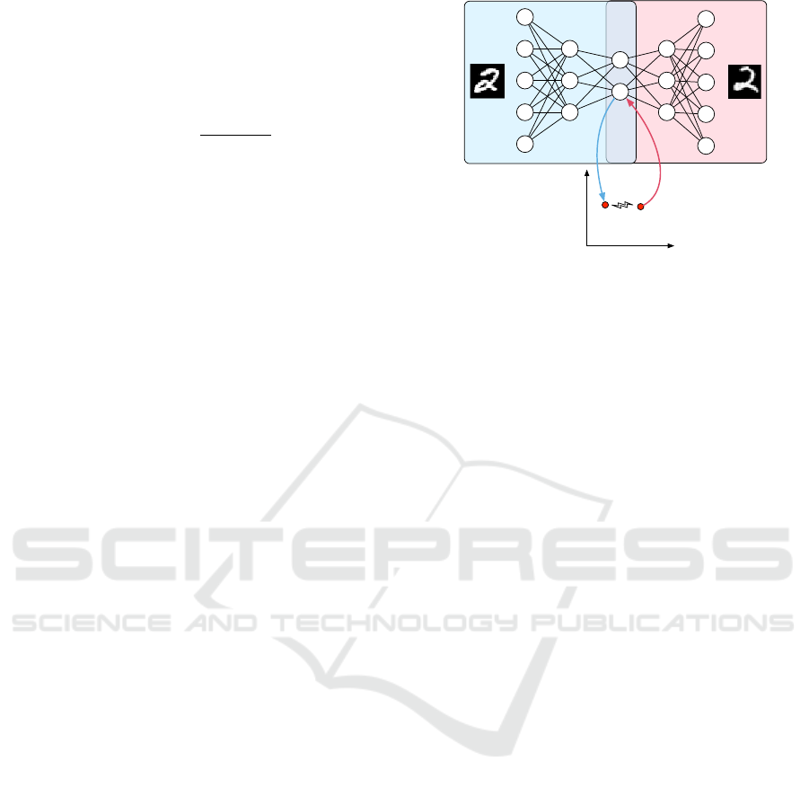
again. A summary of this process is represented in

Figure 1.

t+1

Figure 1: From left to right: the encoder encodes the image

into the latent space, providing a vector z

. Then, perform-

ing some perturbation over this vector, we get the altered

version z

t+1

. Finally, we decode the last vector into a new

image, that would be a modiﬁed version of the original in-

put.

3.2 Generation Methods

Regarding the modiﬁcations that will be carried out

in the feature vectors, we want to evaluate the same

methods as (DeVries and Taylor, 2017): adding noise,

interpolation and extrapolation.

To add noise to the latent vectors, we have used

the following formula:

(i)

= z

(i)

+ αX, X v N {0, σ

}

(8)

Where z

(i)

is the latent vector and

(i)

is the per-

turbed version. We used a 0 mean Gaussian distri-

bution with a standard deviation computed across the

projected dataset. There is an α parameter that con-

trols the inﬂuence of this noise.

Another perturbation that we have evaluated is

the linear interpolation. To do this, we have cho-

sen the three nearest neighbours (kNN with k = 3) in

the feature space, and then we have computed trans-

formations as follows: we have applied for each k

neighbours the following formula, with the parame-

ter α ∈ {0, 1} measuring the contribution:

(i)

= (z

(k)

− z

(i)

)α + z

(i)

(9)

Finally, we have performed extrapolations using

the same nearest neighbours procedure as follows:

(i)

= (z

(i)

− z

(k)

)α + z

(i)

(10)

According to the authors, we have selected an

α = 0.5 in every case, even though in the extrapola-

tion scheme this is unbounded. As regards the param-

eter k in kNN algorithm, we have chosen k = 3 for all

the experiments. This process implies the generation

Empirical Evaluation of Variational Autoencoders for Data Augmentation

of a large number of samples that will be used to train

the classiﬁer.

4 EXPERIMENTS AND RESULTS

We have selected two different datasets: MNIST and

UJIPEN. These sets are handwritten digits captured

and preprocessed, and it could provide us with an idea

of how this approach could help the creation of data

augmentation in computer vision problems.

For the subsequent experiments, we have used the

following algorithms:

• Support Vector Machines (SVM-RBF kernel)

• Nearest Neighbours (kNN)

• Multi-Layer Perceptron (MLP)

Regarding the structure of the MLP, we have used

ﬁve layers with 1024 units each one, with DropOut

and Batch Normalization. We have selected these

models as the baseline because of their simplicity, in

contrast with the more advanced ones based on Neu-

ral Networks with dozens of complicated layers, to

evaluate if these basic models could take advantage

of this synthetic data.

According to the generation process, we have

trained a CNN VAE with the following structure, in

the encoder part: 2 Convolutional layers with a kernel

of 5x5 and a stride of 2 with 16 and 8 channels, re-

spectively. After this, there is a fully connected layer

with 1024 hidden units and ﬁnally the last fully con-

nected with Z hidden units that will conform the la-

tent space. We have mirrored this conﬁguration with

the decoder part. Regarding the dimension of the

latent space, we have evaluated Z ∈ [10, 20, 50, 100]

to check how this is compressed and how many di-

mensions are required for each problem. We have

trained the model using the validation set for each

task, stopping the process when the reconstruction

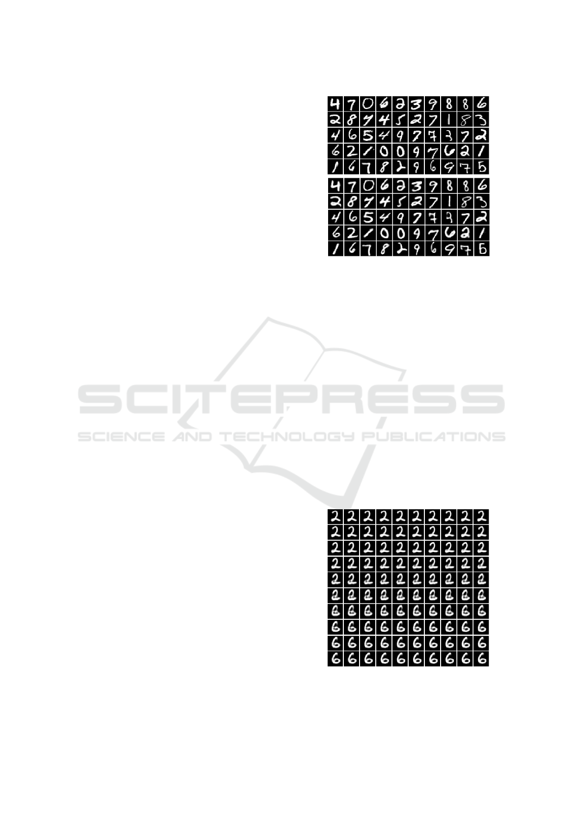
loss increased in validation. The Figure 2 shows some

examples from the ground truth and the reconstructed

digits from the validation set.

4.1 MNIST

One of the most common character dataset,

MNIST (LeCun et al., 1998) is a database of

digits from 0 to 9 which contains 70000 handwritten

images with 28x28 pixels. Even though the error

rate is under 0.5% (Goodfellow et al., 2013) and it

is considered a solved task, this dataset is used as a

sanity check to evaluate new techniques. We have

used this dataset following these conﬁgurations:

Figure 2: Top: Digits from the validation set, Bottom: After

projecting these digits, the reconstruction using the decoder.

• Full dataset: Training the generative model in an

unsupervised way and generating new instances

with the 55k labelled examples, using 5k as vali-

dation and testing with 10k.

• Restricted dataset: Training the generative model

in an unsupervised way with 55k and generating

new ones only with 1k labelled examples, using

5k as validation and testing with 10k.

With this set up we want to evaluate, ﬁrstly, the

convergence of the model training with the whole

dataset, and secondly, the improvement simulating

the scarcity of instances, limiting the amount of la-

belled data that will be used to generate new samples.

An example of the interpolation that the model can

produce is shown in Figure 3. This example is illus-

trating that even between different classes, the model

can infer and preserve some characteristics of the two

Figure 3: Example of linear interpolation between two

points in the latent space, corresponding to the numbers 2

and 6, and the reconstruction of the computed points in be-

tween.

VISAPP 2018 - International Conference on Computer Vision Theory and Applications

100

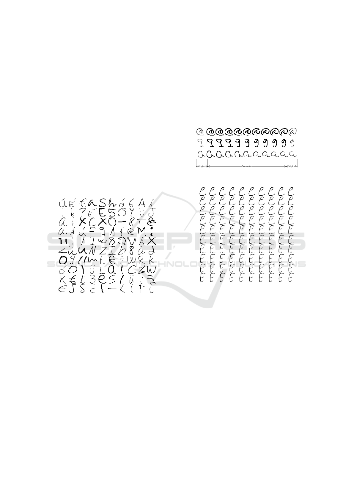
numbers that are involved in the interpolation.

The results of the previous experiments are com-

piled in Table 1 and Table 2, regarding accuracy over

the test partition, considering different dimensions in

the latent space and performing the three methods of

generation. We have not included the results training

with the feature vectors because of the poor accuracy

that they have provided with these classiﬁers. Con-

sidering this, we have continued the experimentation

using just the reconstruction of the feature vectors af-

ter distorting them.

4.2 UJIPEN

The UJI pen character database (Llorens et al., 2008)

is a set of handwritten characters that consists of

grayscale images with a resolution of 70x70 pixels.

It is provided with the information at stroke level, but

they are not used in this work. Some examples of this

dataset could be seen in the Figure 4.

Figure 4: Characters from UJIPEN dataset.

This dataset has two versions, one consisting of

a set of 26 ASCII letters (lower and uppercase) and

10 digits (from 0 to 9). It was created using 11 writ-

ers from Universitat Jaume I (UJI). There is a second

version that adds 49 writers from UJI and Universitat

Polit

ecnica de Val

encia (UPV).

The whole dataset comprises the following char-

acters:

• 52 ASCII letters (lower and uppercase).

• 14 Spanish non-ASCII letters:

N, vowels with

acute accent,

u and

• Digits from 0 to 9.

• Punctuation and other symbols, such as: . , ; : ? !

’ ’ ( ) % - @ <>$.

The choice of this dataset is based on the limited

number of per-class instances. It has 97 classes with

120 samples per label, 11640 in total. We have di-

vided the dataset on 50% for training, 5% for valida-

tion and 45% for testing.

The results of these experiments are shown in Ta-

ble 3. Different examples are shown in Figure 5 and

Figure 6 that illustrate the model’s capacity to inter-

polate between different classes. It is important to re-

mark that the samples generated are a mix between

the source characters, providing the desired variabil-

ity.

Figure 5: Example of linear interpolation between pairs of

characters: “@”, “9” and “a”.

Figure 6: Example of linear interpolation between the char-

acter “e” and “E”.

In the Figure 7 we have included examples of the

generation process using the different methods with

MNIST and UJIPEN.

5 DISCUSSION

We have evaluated the effectiveness of training a gen-

erative model using unlabelled data and then gener-

ate new instances in various models. According to

this, we have validated that the proposed procedure

can help the generalisation of these models, regarding

accuracy’s improvement.

As regards which space is the most appropriate,

we have concluded that when we trained the classi-

ﬁers using the reconstructed generated instances, we

obtained better results than using feature vectors. This

conclusion differs from (DeVries and Taylor, 2017)

Empirical Evaluation of Variational Autoencoders for Data Augmentation

101

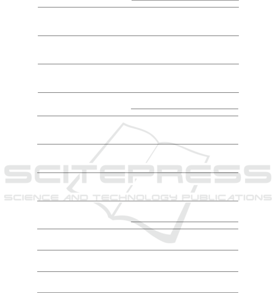
Table 1: Full MNIST results.

Generation methods

Classiﬁer Baseline # of dims. Noise Interpolation Extrapolation

SVM 96.76 100 97.06 96.94 97.43

50 97.08 96.97 97.31

20 96.94 97.18 97.49

10 96,77 97.22 97,56

KNN 96.88 100 95.90 97.28 95.50

50 96.20 97.35 95.49

20 96.06 97.32 96.20

10 95,59 97,31 96,76

MLP 98.39 100 98.12 98.32 97.97

50 98.29 98.18 98.09

20 97.88 98.40 98.29

10 97.62 97.90 98.11

Table 2: Restricted MNIST results.

Generation methods

Classiﬁer Baseline # of dims. Noise Interpolation Extrapolation

SVM 90.00 100 90.64 91.46 91.16

50 90.76 91.44 91.06

20 90.53 91.64 92.27

10 90.83 91.87 91.95

KNN 87.57 100 88.28 91.61 84.51

50 87.83 91.26 83.44

20 87.39 91.53 85.83

10 88.08 91.42 86.95

MLP 90.01 100 87.53 91.49 90.21

50 89.47 91.42 87.26

20 89.73 91.86 89.15

10 89.74 91.61 89.21

Table 3: UJIPEN results.

Generation methods

Classiﬁer Baseline # of dims. Noise Interpolation Extrapolation

SVM 54.79 100 60.18 63.00 63.99

50 59.11 64.68 64.20

20 59.09 63.48 63.19

KNN 31.86 100 41.42 51.34 43.26

50 41.24 50.94 44.44

20 39.29 53.15 46.74

MLP 63.99 100 60.25 61.84 62.62

50 59.41 64.30 60.90

20 57.20 65.60 64.09

where the projected version of the input provided bet-

ter accuracy. These differences could be related to

the use of another kind of generative network, in this

case an LSTM instead of a CNN. The fact that we got

better results reconstructing the distorted versions as

if we were modifying the image agrees with the con-

clusions provided in (Wong et al., 2016), where they

found that the accuracy is improved when performing

variations in the original space rather than in the latent

space.

Differently from (DeVries and Taylor, 2017) we

have found extrapolation useful after reconstructing

the feature vector under certain classiﬁers, such as

SVM or MLP. We have concluded that the room for

improvement is higher in the classiﬁers that are not

based on Neural Networks, such as SVM and kNN. In

these cases, the differences were always signiﬁcant.

Regarding MLP, we have obtained an improvement

VISAPP 2018 - International Conference on Computer Vision Theory and Applications

102

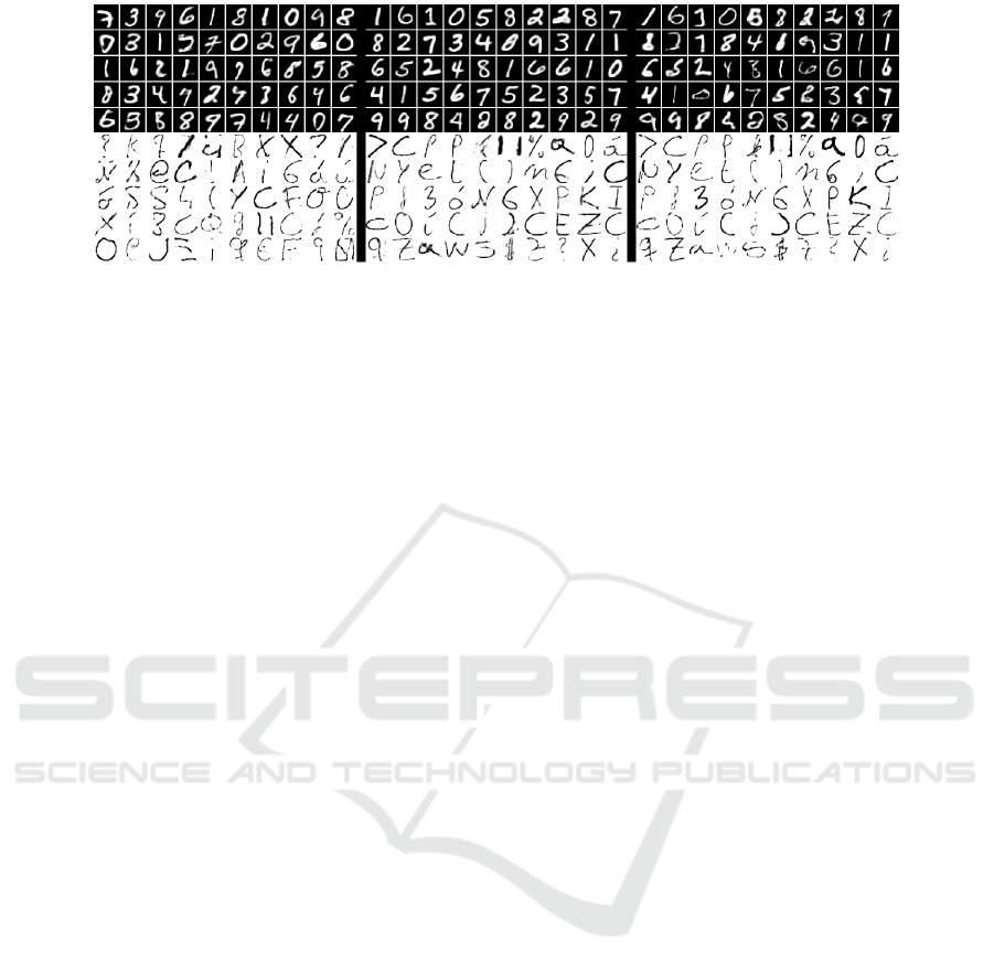
Figure 7: Examples generated with MNIST (top) and with UJIPEN (bottom ) using (from left to right) noise addition, inter-

polation and extrapolation.

but not as remarkable as in the other classiﬁers.

In absolute terms, adding noise has provided the

worst results, while interpolation and extrapolation

had similar ﬁgures when we used SVM. When the

classiﬁer was an MLP with a problem composed of

a signiﬁcant number of classes, as UJIPEN, the dif-

ferences are remarkable, being interpolation the best

method. In the case of MNIST, the improvement

is limited. Visually, interpolation provides examples

with certain ﬁdelity to the real ones while extrapo-

lation generates samples that are different from real

instances. Intuitively, obtaining samples that are far

from the ones in the dataset would have a conse-

quence concerning the accuracy, but according to our

experiments, interpolation has resulted in the best op-

tion.

6 CONCLUSIONS

In this paper, we have evaluated the use of synthetic

data generated by a Neural Network, particularly a

Convolutional VAE, to improve the performance of

different classiﬁers. After projecting the instances in

the latent space learned, we have considered various

ways of generating new instances, such as interpolat-

ing, extrapolating or adding noise to these projected

examples. Once these samples have been modiﬁed,

we have evaluated the performance of decoding the

latent vector or using them directly. We have found

that the best improvement is achieved when the latent

projection is reconstructed.

According to the use of only the original data with

or without the synthetic set, our experiments have

shown that the accuracy improves when this data is

included, paving the way for using this kind of tech-

niques to increase the number of instances when they

are limited.

As a future work, we are considering the use of

these methods in datasets that are not based on im-

ages, such as word embeddings or vectors composed

of features with different nature, where performing

data augmentation manually could be complicated.

ACKNOWLEDGEMENTS

This work was developed in the framework of the

PROMETEOII/2014/030 research project “Adaptive

learning and multimodality in machine translation

and text transcription”, funded by the Generalitat Va-

lenciana. The work of the ﬁrst author is ﬁnanced by

Grant FPU14/03981, from the Spanish Ministry of

Education, Culture and Sport.

REFERENCES

Chawla, N. V., Bowyer, K. W., Hall, L. O., and Kegelmeyer,

W. P. (2002). Smote: synthetic minority over-

sampling technique. Journal of artiﬁcial intelligence

research, 16:321–357.

DeVries, T. and Taylor, G. W. (2017). Dataset augmentation

in feature space. arXiv preprint arXiv:1702.05538.

Goodfellow, I., Pouget-Abadie, J., Mirza, M., Xu, B.,

Warde-Farley, D., Ozair, S., Courville, A., and Ben-

gio, Y. (2014). Generative adversarial nets. In

Advances in neural information processing systems,

pages 2672–2680.

Goodfellow, I. J., Warde-Farley, D., Mirza, M., Courville,

A., and Bengio, Y. (2013). Maxout networks. arXiv

preprint arXiv:1302.4389.

He, K., Zhang, X., Ren, S., and Sun, J. (2016). Deep resid-

ual learning for image recognition. In Proceedings of

the IEEE conference on computer vision and pattern

recognition, pages 770–778.

Kingma, D. P. and Welling, M. (2014). Stochastic gradi-

ent vb and the variational auto-encoder. In Second In-

ternational Conference on Learning Representations,

ICLR.

Krizhevsky, A., Sutskever, I., and Hinton, G. E. (2012). Im-

agenet classiﬁcation with deep convolutional neural

networks. In Advances in neural information process-

ing systems, pages 1097–1105.

Empirical Evaluation of Variational Autoencoders for Data Augmentation

103

LeCun, Y., Bottou, L., Bengio, Y., and Haffner, P. (1998).

Gradient-based learning applied to document recogni-

tion. Proceedings of the IEEE, 86(11):2278–2324.

Ledig, C., Theis, L., Husz

ar, F., Caballero, J., Cunning-

ham, A., Acosta, A., Aitken, A., Tejani, A., Totz, J.,

Wang, Z., et al. (2016). Photo-realistic single image

super-resolution using a generative adversarial net-

work. arXiv preprint arXiv:1609.04802.

Li, X. and Wu, X. (2015). Constructing long short-

term memory based deep recurrent neural networks

for large vocabulary speech recognition. In Acous-

tics, Speech and Signal Processing (ICASSP), 2015

IEEE International Conference on, pages 4520–4524.

IEEE.

Llorens, D., Prat, F., Marzal, A., Vilar, J. M., Castro, M. J.,

Amengual, J.-C., Barrachina, S., Castellanos, A., Bo-

quera, S. E., G

omez, J., et al. (2008). The ujipenchars

database: a pen-based database of isolated handwrit-

ten characters. In LREC.

Rumelhart, D. E., Hinton, G. E., and Williams, R. J. (1985).

Learning internal representations by error propaga-

tion. Technical report, California Univ San Diego La

Jolla Inst for Cognitive Science.

Schl

uter, J. and Grill, T. (2015). Exploring data augmenta-

tion for improved singing voice detection with neural

networks. In ISMIR, pages 121–126.

Srivastava, N., Mansimov, E., and Salakhudinov, R. (2015).

Unsupervised learning of video representations using

lstms. In International Conference on Machine Learn-

ing, pages 843–852.

Wong, S. C., Gatt, A., Stamatescu, V., and McDonnell,

M. D. (2016). Understanding data augmentation for

classiﬁcation: when to warp? In Digital Image Com-

puting: Techniques and Applications (DICTA), 2016

International Conference on, pages 1–6. IEEE.

VISAPP 2018 - International Conference on Computer Vision Theory and Applications

104