
Model-Based Development of Self-Adaptive Autonomous Vehicles using
the SMARDT Methodology
Steffen Hillemacher
1
, Stefan Kriebel
2
, Evgeny Kusmenko
1
, Mike Lorang
1
, Bernhard Rumpe
1
,
Albi Sema
1
, Georg Strobl
2
and Michael von Wenckstern
1
1
Software Engineering, RWTH Aachen University, Germany
2
BMW Group, Germany
Keywords:
Reference paper for SMARDT methodology in Automotive Industry, Elf-driving Vehicles, Modeling
Languages.
Abstract:
Cyber-physical systems are deeply intertwined with their corresponding environment through sensors and ac-
tuators. To avoid severe accidents with surrounding objects, testing the the behavior of such systems is crucial.
Therefore, this paper presents the novel SMARDT (Specification Methodology Applicable to Requirements,
Design, and Testing) approach to enable automated test generation based on the requirement specification and
design models formalized in SysML. This paper presents and applies the novel SMARDT methodology to de-
velop a self-adaptive software architecture dealing with controlling, planning, environment understanding, and
parameter tuning. To formalize our architecture we employ a recently introduced homogeneous model-driven
approach for component and connector languages integrating features indispensable in the cyber-physical sys-
tems domain. In a compelling case study we show the model driven design of a self-adaptive vehicle robot
based on a modular and extensible architecture.
1 INTRODUCTION
In the exciting field of self-driving vehicles devel-
opers and researchers have been faced with a vari-
ety of interdisciplinary problems from areas such as
control theory, electrical and mechanical engineering
as well as computer science for many years (Urm-
son et al., 2008). Obviously, efficient development
of autonomous driving systems is only possible by
means of elaborated methodologies, languages, and
tools providing a high level of automation (Baheti and
Gill, 2011).
The complexity problem in automotive industry
affects different phases and elements of system de-
velopment, especially the specification of the require-
ments, the design and the architecture of the systems
as well as their integration and testing (Grimm, 2003).
Right now, the V-Model approach is used to create
requirements and informal design as well as specifi-
cation or functionality models on the left side for the
system in different abstraction layers. Each layer on
the left side has a corresponding testing step on the
right side in the V-Model. But the development and
maintenance (e.g. due to feature evolution) of these
tests are done manually most of the time. This leads to
several disadvantages: (1) the test model on the right
side may become inconsistent to its original specifi-
cation on the left side, (2) updating the specification
requires an update of all handwritten tests this specifi-
cation links to, (3) due to time pressure, often only the
functionality on the lower layers is updated, whereas
requirements and design specification of the layers
above become inconsistent with the updated behav-
ior, which may lead to misunderstandings inside the
team and make the documentation obsolete, (4) the
SysML specification is so general (Liang et al., 2004)
that different teams in a company may interpret or un-
derstand these diagrams semantically differently.
To overcome all of these shortcomings, the
SMARDT approach (Specification Methodology Ap-
plicable to Requirements, Design, and Testing) uses
only a strict and formalized subset of SysML dia-
grams so that for each layer test cases can be derived
automatically to test whether the developed system
satisfies the specification of each layer. This enables
higher consistency between different abstraction lay-
ers of the V-Model when using an agile development
process.
This Reference Paper Introduces the Novel
SMARDT Methodology with its Focus on Algo-
Hillemacher, S., Kriebel, S., Kusmenko, E., Lorang, M., Rumpe, B., Sema, A., Strobl, G. and Wenckstern, M.
Model-Based Development of Self-Adaptive Autonomous Vehicles using the SMARDT Methodology.
DOI: 10.5220/0006603701630178
In Proceedings of the 6th International Conference on Model-Driven Engineering and Software Development (MODELSWARD 2018), pages 163-178
ISBN: 978-989-758-283-7
Copyright © 2018 by SCITEPRESS – Science and Technology Publications, Lda. All rights reserved
163

rithms for Deriving Test Cases from Activity Di-
agrams and (Internal) Block Diagrams that are
used to Model the System behavior in the Different
Abstraction Layers. All presented diagram types to
model software in the different layers are explained
in a case study showing the model-based design of a
self-adaptive autonomous racing car tuning its control
parameters after each lap in order to improve its driv-
ing behavior.
Component & Connector (C&C) architectures
have proven to be an appropriate approach for the
domain opening up a data-flow driven and hierar-
chical perspective on the system. Prominent exam-
ples of C&C languages originating from the con-
trol domain are MATLAB Simulink (Mathworks
Inc., 2016), Modelica (Modelica Association, 2005;
Elmqvist et al., 1999), AutoFocus3 (Aravantinos
et al., 2015), LabView (National Instruments, 1998),
Verilog (Accellera SYSTEMS INITIATIVE, 2014),
VHDL (The Institute of Electrical and Electronics En-
gineers, 1988; Ashenden, 2010), JigCell (Palmisano
et al., 2015), and Scade (Dormoy, 2008). They sup-
port the system designer with a broad set of libraries, a
discrete time simulator, as well as efficient code gen-
eration for different targets. However, Cyber-Physical
System (CPS) developers can find themselves con-
fronted with a series of drawbacks when using mod-
ern C&C languages such as the lack of a unit based
type systems, missing component and connector re-
use concepts, as well as an overwhelming user in-
terface. A comparison of state-of-the-art C&C lan-
guages and their shortcomings with the focus on the
CPS domain was given in (Kusmenko et al., 2017).
Furthermore, an integrated and homogeneous model-
driven framework named MontiCAR was introduced
addressing these issues.
This Paper Evaluates MontiCAR inside the
SMARDT Process to Show How MontiCAR Over-
comes the Identified Difficulties of C&C Lan-
guages. As our target we choose OpenDaVINCI, a
middleware which has proven to be an efficient ba-
sis for automated driving applications in recent years
(Berger, 2016). This allows us to generate distributed
and realtime-capable architectures. We then evaluate
and test our models in the widely used Open Racing
Car Simulator (TORCS).
The contribution of this paper are the following:
(1) We present a development process for embedded
systems which is conform with ISO 26262. This pro-
cess consist of four layers: object of reflection (textual
requirements and use cases), logical layer (functional-
ity modeled by abstract C&C models and underspec-
ified activity diagrams), technical concept (determin-
istic C&C models and C-code), and realization (e.g.,
ECUs, CAN-BUS, Flexray, and timing). (2) We eval-
uate MontiCAR as a formal and stream based C&C
modeling language for CPS behavior specification.
(3) We present an algorithm which is capable of cre-
ating a realization model from the concrete techni-
cal concept by binding all configuration parameters.
An evolutionary algorithm is used. (4) Finally, in a
compelling case study we show the design of a self-
adaptive vehicle robot based on a modular and exten-
sible architecture.
The remainder of the paper is structured as fol-
lows: first, a running example is presented in Sec. 2
in order to make the reader familiar with the difficul-
ties arising when developing CPS. Thereafter, Sec. 3
shows the first main contribution, the SMARDT ap-
proach. The second layer of SMARDT is discussed
in Sec. 4. In Sec. 5 the models of the third SMARDT
layer are presented in more detail. Next, Sec. 6
shows how input and output streams for functional
testing of C&C models are generated. The experi-
ments conducted in Sec. 7 underline the feasibility of
the SMARDT methodology. Finally, we conclude our
paper in Sec. 8.
2 RUNNING EXAMPLE
On the physical side, one of the main differences of
an autonomous vehicle compared to a manned one is
the enormous variety of sensors the automated vehicle
needs to be equipped with. These sensors are required
to perceive the environment as accurately as possible.
For example, a GPS receiver senses satellite signals in
order to recover its own position, ultra-sonic transduc-
ers can localize obstacles by measuring ultra-sound
echoes. Complex detection and understanding of ob-
jects and their relationships can be done using cam-
eras and computer vision techniques. On the other
hand, the actuators provide a means to manipulate the
physical state of the vehicle by (1) accelerating, (2)
braking, and (3) steering. The behavior of the vehicle
can now be defined as a computational model map-
ping the vehicle’s goal, its sensor inputs, as well as
other accessible knowledge such as maps to actuator
commands. Ideally, the software developer would not
need to know the technical manufacturer specific de-
tails of the sensors and actuators installed in the ve-
hicle but would rather get a homogeneous access to
all available sensor and actuator data via a common
interface. As a running example for the further de-
velopment we will develop a self-driving racing car
system. Such a vehicle needs to have a precise steer-
ing even for high velocities. On the other hand, no
complex urban situation understanding and decision
MODELSWARD 2018 - 6th International Conference on Model-Driven Engineering and Software Development
164

w
L
Steering of wheel
Car state
Road marker
Planned trajectory
Target point
Car position
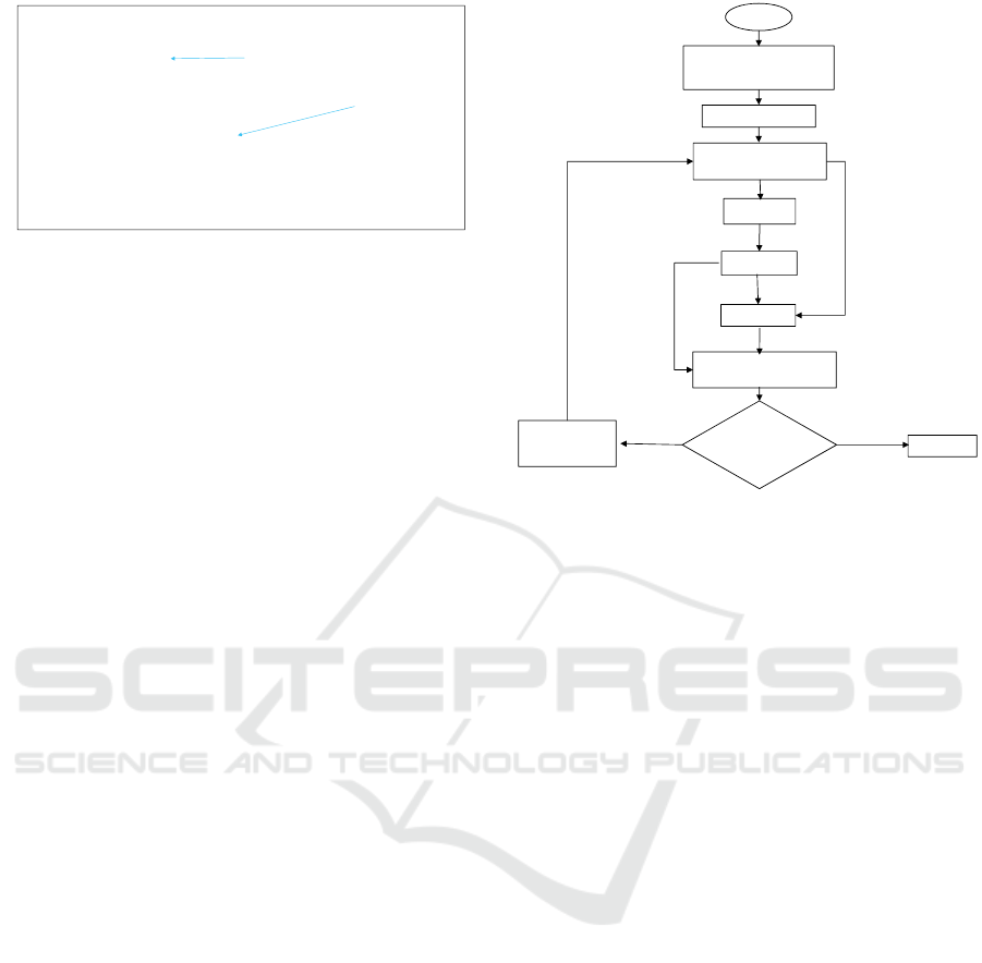
Figure 1: Sketch of the vehicle and main quantities.
making is necessary allowing us to concentrate on the
development of the controller system. We model our
self-driving vehicle as a cuboid of length L, width W
and height H. We assume that the vehicle has full ac-
cess to the map of the track it is driving on. Further-
more we assume, that it possesses a series of sensors
measuring the speed v, wheel angle φ , the position
of the car x as well as its yaw ϕ up to a certain preci-
sion as depicted in Fig. 1. Usually, the behavior of an
autonomous control system is defined not only by the
algorithm or the model but also by a well chosen set of
parameters θ. Often, the optimal parameter set varies
from one physical vehicle realization to another due
to differences in configuration, software evolution but
also random physical factors introduced during manu-
facturing and may even change during the lifetime of
a CPS. Since fine tuning these parameters for every
single vehicle is infeasible due to the high cost, the
vehicle should detect and re-adjust its operating point
on-line.
3 SMARDT METHODOLOGY
With the introduction of ISO 26262, an international
standard for functional safety of road vehicles, the de-
mand for a new specification methodology for safety-
relevant automotive functions arose. As a result,
the Specification Methodology Applicable to Require-
ments, Design, and Testing (SMARDT)
1
was devel-
oped. SMARDT is based on the German V-Model
(Br
¨
ohl and Dr
¨
oschel, 1995), the official project man-
agement methodology of the German government.
In the basic V-Model the left side represents the
decomposition of requirements and creation of sys-
tem specifications. The right side, on the other hand,
represents the integration of developed system parts
and their validation. In general, the V-Model struc-
1
The original abbreviation SMArDT is related to the
German term ”Spezifikations-Methode f
¨
ur Anforderung,
Design und Test”
tures requirements and specifications of a system in
different abstraction layers. Each layer on the left
side has a corresponding testing step on the right side.
However, the creation of these tests is done manually
most of the time. This leads to several disadvantages:
• Ensuring consistency between the tests on the
right side and the specifications on the left side
becomes difficult, since only vague links between
tests and specifications exist.
• Updating the specifications results in the neces-
sity of a manual update of all the corresponding
handwritten tests.
• Extending a system’s functionality is mostly done
only on the lowest layer due to time pressure. Re-
quirements and specifications of the higher layers,
however, are not updated accordingly.
To overcome all of these shortcomings, the
SMARDT approach uses only a strict and formal-
ized subset of SysML diagrams (OMG, 2015) with
a meaningful and clear semantics (Harel and Rumpe,
2004) to specify the functionality of a system. As
a consequence, a higher consistency between differ-
ent abstraction layers of the V-Model is achieved,
especially for agile development processes, which
are mostly iterative, incremental, and evolutionary
(Beck et al., 2001). The rigorous mathematical the-
ory behind the used SysML diagrams enables fur-
ther validations such as (1) backward compatibility
checks (Rumpe et al., 2015; Richenhagen et al., 2016;
Bertram et al., 2016) for software maintenance and
evolution between different diagram versions of the
same layer as well as (2) refinement checks (Rumpe,
1996) between diagrams of different layers for de-
tecting inconsistencies in specifications between dif-
ferent layers, mostly between the first and second
one. This paper’s main focus lies on the testing part
of the SMARDT approach to enable agile modeling
(Rumpe, 2017) in SysML.
In general, SMARDT describes a formal specifi-
cation for requirements, design, and testing of sys-
tem engineering artifacts according to the ISO 26262
specifications, as illustrated in Fig. 2. Four abstrac-
tion layers structure the method:
1. The first layer contains a first description of the
object under consideration and shows its bound-
aries from a customers point of view.
2. The second layer contains functional specifica-
tions without details of their technical realiza-
tions.
3. The third layer embraces the technical concepts of
the system.
Model-Based Development of Self-Adaptive Autonomous Vehicles using the SMARDT Methodology
165
D
1
st
layer
2
nd
layer
Req
Req
D
Sys1
st
D
D
Sys2
nd
Object of reflection
Logical layer
3
rd
layer
Req
D
D
Sys3
rd
4
th
layer
Req
D
D
Code4
th
Technical concept
HW+SW Realization
Req
original
Structural
Refinement Validation
Dx
th
SysML diagrams x
th
layer
Req
Textual Requirements
Trace link
Manual Transformation
Automatically generated
Product
Artifact
deployment
Test1
Test1’
Test1’’
Test1’’’
Test1’’’
Test2
Test2’
Test2’’
Test2’’’
Test3
Test3’
Test3’’
Test4
Test4’
product
Automatically transformed
New in
SMARDT
Classical
V-Model
Figure 2: Overview of the SMARDT methodology.
4. The fourth layer represents the software and hard-
ware artifacts present in the system’s implementa-
tion.
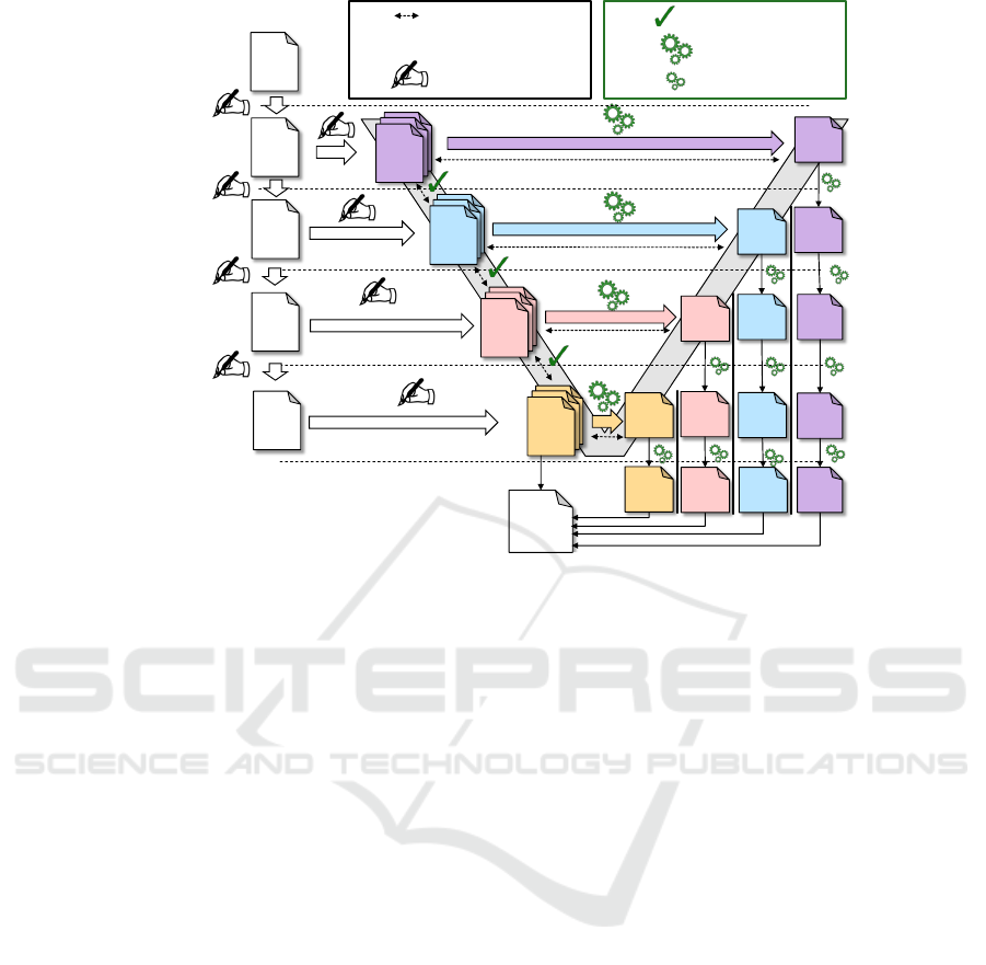
As depicted by Fig. 2, SMARDT achieves a
higher consistency between the different layers by
verifying and model-based testing (Philipps et al.,
2003) that the final product meets the requirements of
all layers. More specifically, SMARDT enables struc-
tural verification as discussed in (Bertram et al., 2017)
between each layer indicated by the green check
marks in Fig. 2. Furthermore, SMARDT enables a
systematic and fully automatic derivation of test cases
for each layer by allowing only a formalized subset of
SysML diagrams on each layer (Rumpe, 2003). Fi-
nally, SMARDT ensures consistency between the test
cases of each layer by enforcing that the test cases
of one layer can also be used on the lower layers by
transforming them. This is illustrated on the right side
of Fig. 2. For instance, layer 1 describes functional-
ity of the product on the highest level. Hence, the
corresponding test cases cannot be used directly on
the lower layers, and therefore must be transformed to
multiple low-level test cases (Pretschner et al., 2004).
This is done, for instance, by substituting abstract sig-
nal names and values with concrete hardware signals
and values.
The first two abstraction layers are conceptual in
the sense that their diagrams lack a direct counter-
part in the implementation. The behavior modeled
within the diagrams can later be implemented across
several components. Moreover, signals used in these
diagrams are logical, i.e., they abstract away from
signals of the implementation. Consequently, corre-
sponding values comprise a range of values present
in the implementation. In contrast, the elements of
the third and fourth layers have a direct representa-
tion within the implementation. The third layer de-
scribes hardware-independent functionality of a sys-
tem, whereas the fourth layer contains software parts
that are specific to a given micro-controller and also
handles low-level behavior such as I/O-interrupts.
A lot of research about improving and tailoring the
V-Model to company-specific needs at management
level has been conducted (V-Modell XT, 2006; Broy
and Rausch, 2005; Friedrich et al., 2009). In contrast
to these works, the SMARDT methodology focuses
not on integrating the process into different business
structures but rather on the formal and technical parts
of the specification diagrams of the different layers
in the V-Model to have a traceable, verifiable, consis-
tent, and particularly, testable artifacts over the entire
development process.
The rest of this paper applies the SMARDT
methodology for developing a self-adaptive au-
tonomous vehicle. Fig. 3 shows how the original re-
quirement of a superior driving experience is step-
wise refined to concrete technical ones. Each layer re-
fines the requirements of the higher layers by adding
more details. Starting with the original requirement
R1, each layer subdivides this requirement into more
MODELSWARD 2018 - 6th International Conference on Model-Driven Engineering and Software Development
166
specific ones. Consequently, SMARDT enables trac-
ing the requirements through all layer. Moreover,
Layer 3 is divided into 3A (generic technical concept)
and 3B (concrete technical concept). The generic
technical concept presents a functional architecture
with unbound configuration parameters, while in con-
trast the concrete technical concept binds all the con-
figuration parameters. In this way the architecture of
layer 3A can be reused in different model series. Dif-
ferent car engines, dimensions, weights, and wheel-
bases but also variations in the manufacturing process
are reasons why cars expose different behaviors in
their environment. Hence, no general controller exists
and car-specific parameters must be derived in Layer
3B.
4 ACTIVITY DIAGRAMS FOR
SMARDT LAYER 2
We present a version of SysML activity diagrams ex-
hibiting formal expressions (Maoz et al., 2011). Us-
ing these expressions we are able to provide detailed
specifications of the functionality modeled on the sec-
ond layer of SMARDT. Although these high level
specifications are independent of the technical con-
cept, they still can be used to describe abstract system
constraints without predetermining the way they have
to be implemented.
For formal expressions we use the OCL/P spec-
ification language (Rumpe, 2016), which is a Java-
based OCL derivate. OCL is well suited for
implementation-independent high level specifications
describing system constraints (Gogolla et al., 2007).
R1: Self-Driving Racing car offers
superior autonomous driving experience.
R4: Trajectory lies in the middle of the
lane
R5: Trajectory begins at vehicle position
R6: Vehicle follows calculated trajectory
R7: Vehicle tracks the laps driven
R8: Vehicle tracks the MSE for each lap
R9: At the end of each lap, car adapts its
behavior to improve the MSE
R10: Car computes trajectory error
R11: Car controls steering actuator to
follow the trajectory
R12: Car controls braking and
accelaration to achieve the required
speed
R13: Mean squared error must be below
car-specific threshold
R14: Max. error must be below
environment-specific threshold
R15: Distance to car in front is at least 2m
original
Layer 2
Layer 3A
Layer 3B
Layer 1
R2: Car drives 20 laps on a given track.
R3: Car assesses and adopts its behavior.
Req
Generic technical
concept
Concrete technical
concept
Logical layer
Object of reflection
«refines R2»
Req
Req
Req
Req
«refines R3»
«refines R6»
«refines R7»
Figure 3: Requirement refinement in a simplified SMARDT
process.
Map
(Lists of left, right lane
markers)
Location
Plan trajectory
Goal
Trajectory
!
"#$
"
%
$
Check new
Lap started
prevLocation
&'()
* %
+,'()-
-
."/0)
* %
+1"/0)-
23
/45&
6 * 6
$
&'()
7
."/0)
8
&'()
8
96
:
&'()
8
;9
."/0)
7
&'()
7
;-
("<"=0'>
?
3%--23
/45&
@% -A ? 3%--23
/45&
% B
23
/45&
%
-
prevParam
Param
Compute
Controls
[A
("<"=0'>
]
Evaluate
Lap MSE
("<"=0'>
C
,5+
? C
,5+
)4)5&
? D% 3
C,5+E$
--
3
C,5+
? D%
% ?
F %-% C
,5+
? % ? G
Adapt
Param
<
* -%
&,'().1"/0)
%
% ? %
currentTime
Diagram is executed
every
H
seconds
IJK ?
$
L
MNMOP
Q
<
:
<
R H-
IJK S 32-TT
C
,5+
!
U V @U
ControlCommand
U ? @U
Keep
Param
3!
ExecuteCarLogic
W
WW
W
X
XX
X
Y
YY
Y
Z
ZZ
Z
[
[[
[
\
\\
\
]
]]
]
^
^^
^
_
__
_
`
``
`
a
aa
a
b
bb
b
c
cc
c
d
dd
d
e
ee
e
Decision node
Merge node
Input ports
Activity
Data flow
Control flow
Guard condition
Output specification
Figure 4: Activity diagram describing the car logic executed
in each time step.
Another benefit of OCL/P is its extension for units
(Maoz et al., 2017), making it even more suited for
embedded systems.
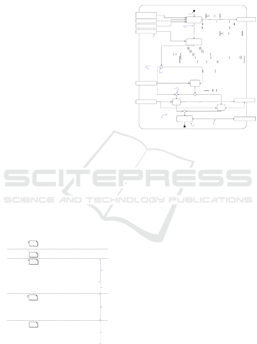
Example Activity Diagram. To show how OCL/P
is used, Fig. 4 illustrates a simplified activity diagram
(AD) describing the car logic. In general, the struc-
ture of the ADs used on the second layer of SMARDT
is similar to the SysML standard. Inputs and outputs
of the function are modeled using ports. Besides the
control flow, the object flow of a diagram explicitly
indicates when and where the information is passed.
Action nodes are used to model single steps of the
function. Control nodes, e.g., decision nodes, model
any decision logic and parallelism of a function. For
the description of the former we added OCL/P expres-
sions to the diagrams. As These expressions are used
as guards, but also to extend the control flow edges.
Without loss of generality and for better readability
we use pure mathematical expressions for the formal
specification in Fig. 4. However, this notation can eas-
ily be translated to OCL/P as will be shown in the fol-
lowing. This way, each edge not only models the con-
trol flow of an AD, but can also be used to build up an
OCL/P expression. For instance, the outgoing edge of
the action Check new lap started contains a for-
mal expression providing several definitions and an
assignment. The newly assigned Lap
f inished
is used in
the guards of the following decision node. Depending
on its evaluation different actions are performed next.
As the example AD of Fig. 4 demonstrates, by ex-
Model-Based Development of Self-Adaptive Autonomous Vehicles using the SMARDT Methodology
167
tending ADs with formal logics we are able to model
powerful formal expressions within a diagram. These
expression can be used as high level specifications to
describe abstract system constraints as well as a basis
for automated test case derivation.
As is common for embedded systems, the de-
signed software of our example is executed in three
phases: (1) the initialization phase, (2) the main loop,
and (3) the exit phase. At system initialization the
lap and cycle counters are set to zero. In the main
loop the activity diagram is executed in every time
step thereby exhibiting the following behavior. First,
the trajectory is computed based on the abstract map
(represented by two lists of left and right lane mark-
ers, respectively), the vehicle’s goal, and its current
location. Thereby, the resulting trajectory has to ful-
fill the following constraints:
•
1 The trajectory does not deviate by more
than 0.25m from the road middle line which
can be formalized in OCL/P as forall p in
Trajectory: exists l in Left, r in Right:
norm(0.5*(l+r)-p)<= 0.25m.
• 2 The discrete trajectory consists of points,
which are at most 0.5m apart: forall i in 1 ..
Trajectory.size - 1: norm(Trajectory[i+1]
- Trajectory[i]) <= 1m.
• 3 The first trajectory point is within a ra-
dius of 0.25m from the current car position:
norm(Location - Trajectory[1]) <= 0.25m.
Apparently, OCL/P is close to the pure mathemati-
cal notation provided in Fig. 4. Once the trajectory
is computed, 4 the error which is defined as the dis-
tance between the car and the road middle line is com-
puted for later evaluation and 5 the cycle counter is
incremented. The car checks whether it just started
a new lap by 6 analyzing if it crossed the line be-
tween the left and right road markers closest to the
goal. If 7 a new lap is started, 8 the lap counter is
incremented, 9 the total lap time for the finished lap
is computed, 10 the start time of the new lap is set,
and 11 the cycle counter is reset. Then 12 the mean
squared error (MSE) for the finished lap is computed.
If 13 the MSE is above a specified threshold and the
car has not finished a total of 20 laps, the parameters
are adapted and 15 must differ from the old ones. Oth-
erwise the old parameter set is kept 14 . Finally, the
control commands are computed and outputted termi-
nating the execution cycle.
It is also possible to specify well-formedness rules
(such as stability, smoothness, and responsiveness
(Matinnejad et al., 2017; Slicker and Loh, 1996)) for
the output ports (e.g. ControlCommands) of closed-
loop-control systems. An example of a smoothness
Left lane markers
Right lane markers
Trajectory
Goal
0.5m tube around road middle line
Current Position
Input Values n Trajectory Lap
finished
#Lap MSE Param
200 false 5 N/A
0 true 6 MSE >
Threshold
1 false 6 N/A
expected output and internal values
Figure 5: Exemplary test case derived from the AD in
Fig. 4.
rule specified in OCL/P could be that the difference
of two successive steering control commands should
be smaller than two degrees.
Deriving Test Cases from Activity Diagrams. Be-
sides providing high level specifications, introducing
formal OCL/P expressions to activity diagrams (ADs)
also enables a systematic derivation (Mingsong et al.,
2006) of test cases. The output of the derivation pro-
cess are test cases, which can be used to test the func-
tional specifications modeled by the ADs.
The basic approach for the derivation of test cases
consists of several steps. First, the interface of the
AD, respectively the modeled function, is determined.
This can easily be done, since inputs and outputs are
modeled explicitly in the AD by ports. Second, the set
of paths through the diagram fulfilling the path cov-
erage criterion C2c (Liggesmeyer, 2009), with each
loop iterated once, is calculated. Based on this set,
for each path a formal expression is built. This is done
by analyzing each edge of the path and extracting the
OCL/P expression. Third, for a set of initial condi-
tions, the AD can be executed an arbitrary number of
times and depending on the current input values the
expected output and internal values can be calculated.
During the calculation, the OCL/P expression of the
specific path through the AD is evaluated. In the end,
the resulting test case consists of a sequence of evalu-
ated execution cycles.
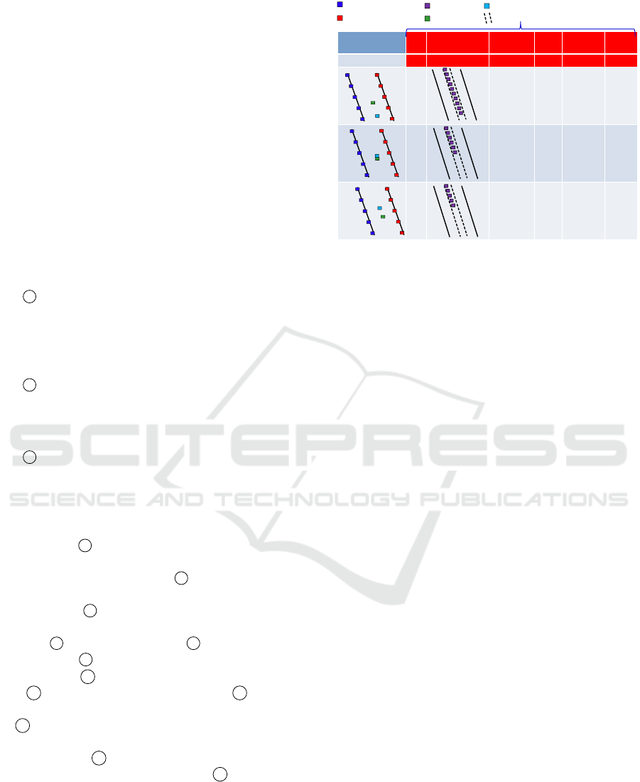
Fig. 5 presents an excerpt of an exemplary test
case in form of a table derived from the AD shown
in Fig. 4. The excerpt shows a test sequence between
lap 5 and 6. Each row represents one execution of
the AD. For better readability the input values as well
as the trajectory are presented graphically instead of
concrete values. For the input values differently col-
ored markers are used depicting the map, i.e., left lane
MODELSWARD 2018 - 6th International Conference on Model-Driven Engineering and Software Development
168

and right lane, the current position of the car, and the
goal. The expected output and internal values are to
the right of the column containing the input values.
The expected output and internal values include, for
instance, the current lap and parameter set of the re-
spective diagram execution. Given the input values of
each execution, the expected values are calculated by
evaluating the OCL/P expression of the path through
the diagram.
The derived test cases for the ADs of SMARDT
layer 2 can be transformed to test cases for the fol-
lowing layers. Note that since the ADs of layer 2 only
model the functional specifications without details of
their technical realizations, the abstract signal names
used in the ADs need to be mapped to the concrete
technical signals used on the lower layers. As shown
in Fig. 2 test cases for layer 3, layer 4, and the final
product are generated based on the activity diagram.
The test cases of layer 3 allow early detection of func-
tional errors to avoid inconsistencies as early as pos-
sible. While the test cases for layer 4 ensure that the
Hardware/Software integration did not introduce any
functional incorrectness (e.g. variable overflow), the
test cases for the final product ensure that the cus-
tomer experience is as it is described in the activity
diagram.
5 COMPONENT AND
CONNECTOR MODELS FOR
SMARDT LAYER 3
Existing Approaches to Model Self-Driving Cars.
Self-driving vehicle architectures have been discussed
in several works. In (Montemerlo et al., 2008) a mod-
ular architecture which proved to be successful in the
DARPA urban challenge was proposed. It consists of
four layers, namely, the sensor interface, perception,
navigation, and a user / vehicle interface. A series of
heterogeneous sensors enable the vehicle to perceive
its environment. A similar approach dividing the ar-
chitecture into perception, behavior and planning is
presented in (Wei et al., 2013). It enables the vehicle
to cope with different kinds of situations by allowing
to integrate a variety of intelligent behaviors. A com-
mon issue with the presented architectures are high
sensor costs. This issue has been addressed, e.g., by
Daimler in the Autonomous Bertha project (Ziegler
et al., 2014) where a cheaper computer vision based
approach was evaluated. Deep learning approaches
have been emerging in the last years, trying to mimic
a human driver by learning from image examples, i.e.,
only requiring camera inputs. In the end-to-end learn-
ing approach, the network tries to predict the best ac-
tuator commands directly after seeing the image (Bo-
jarski et al., 2016). On the other hand, the goal of
the direct perception architecture discussed in (Chen
et al., 2015) is to let a neural network extract features
such as distance to the front car from an input image.
Then, the predicted feature set is passed to a conven-
tional controller in order to generate actuator inputs.
In the domain of control Simulink (Mathworks
Inc., 2016) is one of the dominating C&C frame-
works. Simulink lacks a unit based type system but
provides a variety of static analysis features, matrix
support, and a large component library. Further rel-
evant C&C languages, often specialized to a par-
ticular domain include LabView (test, measurement
and control domain) (National Instruments, 1998),
SysML (systems engineering domain) (OMG, 2015),
VHDL (integrated circuit domain) (The Institute of
Electrical and Electronics Engineers, 1988), Mod-
elica (Modelica Association, 2005) and others. A
detailed overview and comparison is given in (Kus-
menko et al., 2017).
Overall Architecture. An overview of the scenario
we are going to develop in this section is depicted in
Fig. 6. The plant we are using to evaluate our system
is a TORCS vehicle residing inside the simulator on
the left hand side of the figure. The actual self-driving
functionality resides in the driving module including
sensor signal filtering, trajectory planning, as well as
a closed loop controller aiming to fulfill the vehicle’s
goal as efficiently as possible.
The data adapter provides an interface to read sen-
sor data from the vehicle and write actuator com-
mands thereby decoupling the self-driving software
from the physical vehicle platform. By means of the
filtered sensor data and the trajectory planing com-
ponent, the controller computes the actuating values
which are then sent through the data adapter back to
the vehicle in the simulation.
Often it is necessary to experimentally evaluate
different variants and configurations of a system to
find the optimal solution for a given task. There-
fore, modularity and loose coupling are essential in
the development of CPS. However, a correct struc-
tural model of the controller is neither sufficient to
guarantee a correct behavior of the system nor an ap-
propriate parametrization thereof. As an example,
our controller architecture is based on the classical
and well-studied PID controller the basic behavior of
which can be defined in parallel form as
y(t) = Pe(t) + I
Z
t
0
e(τ)dτ + D
∂e
∂t
. (1)
Model-Based Development of Self-Adaptive Autonomous Vehicles using the SMARDT Methodology
169

d
Driving Module
Parameter Tuner
Physical Vehicle
Vehicle
Sensors
Sensor
signals
nsor
Vehicle
Actuators
Smoothing
filter
Main Controller
Simulation
nsor
Data Adapter
Trajectory
Planning
Actuator
commands
Track Data & Goal
Figure 6: Overall Architecture.
Now, each PID controller instance requires a set of at
least three configuration parameters from a continu-
ous search space. Finding a working set of parame-
ters for a system consisting of a series of PID con-
trollers and other parameterizable components by a
brute force search is therefore infeasible. Thus, an in-
telligent approach to automate the tuning of the PID
parameters is needed. Therefore, an exchangeable pa-
rameter tuning component is attached to the driving
module. Since the parameter tuner and the driving
module only need to exchange a convenient perfor-
mance measure and sets of model parameters, the two
components do not need to know anything about each
other’s implementation allowing a loose coupling and
ensuring modularity.
Alternative Control Strategies. Model Predictive
Control (MPC) has established itself as a popular con-
trol strategy. Using a model, the controller can es-
timate the future state of the robot given a series of
inputs. The goal of MPC is to find a series of con-
trol inputs minimizing the error predicted using this
model. MPC needs to solve an optimization problem
in every time step, which makes the approach com-
putationally intense. Further drawbacks are the need
for an appropriate model of the process and possible
instability (Camacho and Alba, 2013). An alternative
control approach being researched which solves in-
stability issues of MPC and other problems is sliding
mode control (Utkin, 2009).
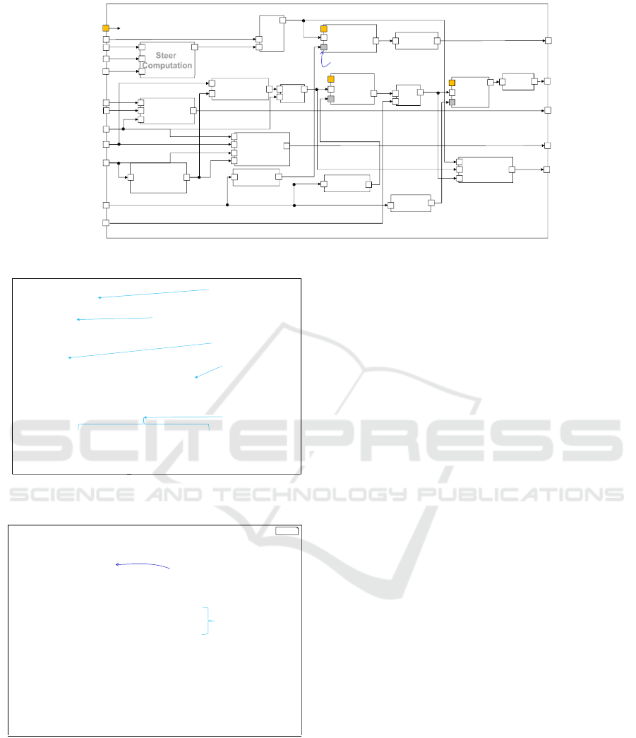
Main Controller. The goal of a closed-loop con-
troller is to compare the state of the plant, including
the vehicle speed and position, measured by the sen-
sors with the desired state and to generate appropri-
ate actuator actions as a reaction to the deviation. In
Fig. 7 the graphical C&C model of the Main Con-
troller is illustrated and will later serve as a basis for
a formal textual model definition in MontiCAR.
For a better readability, only port names and types
of the outer component are given in the figure. Note
that primitive numeric types are denoted by the al-
lowed range of values and in some cases the unit of
the quantity. This high level type system, introduced
in (Kusmenko et al., 2017) allows for a more precise
modeling than by using conventional primitive types
such as integers, floats, and doubles. For instance,
it allows to constrain the maximum speed of the ve-
hicle and to specify the measurement accuracy of its
sensors. Furthermore, it provides means of compat-
ibility checking specific for the CPS domain. As an
example, a speed port cannot be connected to an ac-
celeration port, since the two quantities have differ-
ent unit types. This feature helps preventing logical
errors in the model by appropriate compiler errors.
To keep the model compact, primitive types belong-
ing together such as two-dimensional coordinates and
PID tuples are grouped into structs.
On the left hand side of the diagram input ports
including filtered sensor data as well as PID param-
eters found by parameter tuner are depicted. Further
inputs are track data and the current trajectory goal,
i.e., the next target point. The right hand side shows
output ports for actuating variables as well as an inter-
face to the genetic algorithm. The brake, steering,
gear, and gasPedal values are forwarded to the actu-
ator interface via the data adapter whereas the errors
value is forwarded to the tuner component. The be-
havior of the main controller block is specified by the
interconnection of its subcomponents which are par-
tially taken from a library and partially designed as
primitive components for this case study using Mon-
tiCAR’s math language.
Although the graphical model is well suited to
provide a quick comprehensive overview of the sys-
tem, textual modeling provides several advantages
such as easier version control and collaborative edit-
ing, searching and comparing the models, and others.
An excerpt of the textual MontiCAR model for the
controller architecture is illustrated in Fig. 8.
The component is defined using the component
keyword. It consists of a set of input and output port
declarations as well as a set of subcomponents instan-
tiated using the keyword instance. Finally compo-
nents are reconnected with each other in order to de-
fine the data flow. Thereby, output ports of a compo-
nent can only be connected to type compatible input
ports. Note that the underlying semantics of Mon-
tiCAR is weakly causal, i.e., the computation result
of a component is available instantaneously; neither
computations nor connectors introduce delays.
Before stepping into the details of how the con-
troller output values are computed, the extract compo-
nents are explained. These are needed to understand
how the parameter tuner communicates with the con-
troller. To optimize the parameter values for the three
PID controllers, their parameters need to be passed to
MODELSWARD 2018 - 6th International Conference on Model-Driven Engineering and Software Development
170
steeringMeasured:-45°..45°
gasPedalMeasured: 0..1
targetPos:Point
currPos:Point
carYaw:-180°..180°
currGear:-1..6
carSpecs:carInfo
currVelocity:0..75 m/s
allowedSpeed:0..75 m/s
PIDTupleAggregation:Tuple
roadSpecs:roadInfo[20]
steeringWished:-45°..45°
gasPedalWished:0..1
gear:-1..6
brakePedal:0..1
errors:0:oo
Steer
Computation
-
-
Gear-
Gear
Computation
Gear-
Brake
Computation
Gear-
MaxSpeed
PerSegment-
computation
Gea
PID
steeringPID
Gear-
TargetSpeed
Computation
-
-
Gear-
PID
speedPID
Gear-
PID
accPID
-
-
Gear-
Error
Summation
-
Scale
sSteer
-
Scale
sGas
Extractor
SteerPID
Extractor
SpeedPID
Extractor
AccelPID
Configuration port
time:0 .. ∞ ns
Controller
ControllerController
Controller
…
Figure 7: Main controller component calculating the actuating variables and providing the interface to the genetic algorithm.
The ports of the
components are getting
connected via the keyword
connect and an arrow „->“
component Controller{
ports
in Q(-45° : 0.001° : 45°) steering,
in Point targetPoint,
in Point currPos,
in Q(-180° : 0.001° : 180°) carYaw,
/*other input and out ports*/
instance SteerComputation steerComp;
instance Subtract subtractSteer;
instance PID<°> steeringPID(-45°, 45°, 10°);
connect targetPoint -> steerComp.targetPoint;
connect currPos -> steerComp.currPos;
connect carYaw -> steerComp.carYaw;
connect steerComp.targetSteerAngle -> s
wwed subtractSteer.targetVal;
connect steering -> subtractSteer.measuredVal;
/*Other connectors*/
}
The components are getting
declared with the keyword
instance
2
3
6
7
10
11
12
13
1
4
5
8
9
14
Instantiation of a
parameterized PID with the
bounds -45° and 45°
15
Primitive MontiCAR type
consisting of the number type
(Q=rational, Z=integer,
C=complex), the range and the
resolution
Struct type
Figure 8: MontiCAR code describing the graphical con-
troller model of Fig. 7.
1
component PID<U is Unit>
2
(Q(-oo U:oo U) lower, Q(-oo U:oo U) upper, Q(0 U:oo U) windup){
3
ports in Q(0 s:oo s) time,
4
in Q(-oo U : + oo U) error,
5
in PIDTuple pid,
6
out Q(-oo U :oo U) output;
7
implementation Math {
8
static Q(0 s:oo s) prev_time = time;
9
static Q(-oo U:oo U) prev_error = error;
10
static Q(-oo U:oo U) int_error = 0;
11
Q(0s:oo s) dT = time – prev_time;
12
int_error = int_error + 0.5Hz*dT*(error + prev_error);
13
int_error = max(min(windup, int_error), -windup);
14
T P_term = pid.P*error;
15
T I_term = pid.I*int_error;
16
T D_term = 1s * pid.D*(error – prev_error)/dT;
17
prev_time = time;
18
prev_error = error;
19
output = P_term + I_term + D_term;
20
output = min(max(lower, output), upper);
21
} }
EMA
Initialization part of static
variables takes place only in
first execution cycle
PID parameters can be updated at any time
through the pid port (but should only be updated
when a lap is finished according to requirement R9)
Setting bounded value of the
output port
Figure 9: MontiCAR specification of a PID controller with
an integral windup guard.
the controller as an input. This way, the quality of
the parameter sets can be evaluated during the driv-
ing process. Each PID controller takes three param-
eters, the P-term, the I-term, and the D-term, form-
ing a parameter tuple. To bundle these three parame-
ter tuples for all three PID controllers, a struct called
PIDTupleAggregation is used. In addition, this
struct contains a fitness value which is used later on
by the parameter tuner. The components Extractor
SteerPID, Extractor SpeedPID and Extractor Ac-
celPID are used to extract the right PID parameter tu-
ple from the PIDTupleAggregation struct before be-
ing inputted to the respective PID controller. The con-
troller communicates the following four control vari-
ables to the actuator interface: steering angle, brake
pedal value, gas pedal value, and the gear. To com-
pute these output values there is a need for several
different components. First, the components to calcu-
late the steering angle are outlined.
The SteerComputation component takes the tar-
get position, the current position, and the current car
yaw angle as inputs. By means of these three val-
ues the output steering angle is computed according
to (Bernhard Wymann and Sumner, 2013). In Fig. 10
the definition of the SteerComputation component is
depicted. Here a further example of MontiCAR’s un-
usual type system is provided: the car yaw can only
take values between -180 and +180 degrees with a
resolution of 0.001 degree. The compiler uses this
information for component compatibility checks by
symbolic execution. If a range violation cannot be
detected at compile-time but occurs at runtime, an ex-
ception is thrown by the application. Furthermore,
the unit declaration makes sure the port input is inter-
preted as degrees and not as radiants. If the sender
provides a radiant based version, an automated con-
version takes place. SteerComputation is a primitive
component, i.e., it does not contain any subcompo-
nents and, hence, requires a behavior description pro-
vided here in MontiCAR’s Math language. The latter
uses the aforementioned type system, as well. Fur-
thermore, it provides standard mathematical functions
such as atan as well as integrated support for matrix
Model-Based Development of Self-Adaptive Autonomous Vehicles using the SMARDT Methodology
171

component SteerComputation{
ports
in Point targetPoint,
in Point currPos,
in Q(-180° : 0.001° : 180°) carYaw,
out Q(-45° : 0.001° : 45°) targetSteerAngle;
implementation Math{
Q(-oo : 0.0001 : oo) targetAngle = atan(targetPoint.y –
d currPos.y, targetpoint.x – currPos.x) – carYaw;}
targetSteerangle = targetAngle;
}
}
input values needed for the
of the target steering angle
Setting the output value
min. value max. valueStep size
2
3
6
7
1
4
5
8
9
10
11
Figure 10: The target steering angle is computed by means
of the three input values: targetPoint, currPos and
carYaw. In the end the target steering angle is written to
the output.
operations.
The current steering angle needs to be subtracted
from the target steering angle to get the steering error.
The steering error then acts as one input value of a
PID controller. The other input for the PID controller
is the PID parameter tuple. The PID component is im-
plemented as a parallel structure according to (
˚
Astr
¨
om
and H
¨
agglund, 1995). Its specification is formalized
using MontiCAR in Fig. 9. Note that the unit of
the error to be controlled by the PID may depend on
the application. Therefore, the PID component has a
generic unit parameter U which is a Unit. The latter
is bound to JScience javax.measure.unit.Unit
making it compatible with JSR275 (Dautelle and Keil,
2010). In the implementation part, the keyword
static is introduced. The value of a static Mon-
tiCAR variable remains available when an execution
cycle is finished. Furthermore, the initialization ex-
pression provided with the static variable’s definition
is only evaluated in the first execution cycle. Dynamic
systems such as the PID controller depend not only on
the current inputs but also on the past and, hence, can
be modeled efficiently using this new language con-
struct while superseding the need of memory blocks.
Since the output of a PID component is theoreti-
cally not bounded, we constrain it to have a minimal
and a maximal output value of −45
◦
and 45
◦
, respec-
tively. This is done similar to Simulink by providing
additional parameters to the PID in line 9 of Fig. 8.
In order to compute the fitting acceleration and
braking, information about the road is required. In
TORCS the road is divided into segments. The fol-
lowing properties of the road segments are known and
stored in the map data: length, radius, friction co-
efficient, an enum value capturing the segment type
(straight or curved), as well as the distance to the seg-
ment end to determine where the car is situated in the
current segment. The distance to the segment end at-
tribute equals the length of the segment for every seg-
ment, except the one the car is currently driving on.
These properties are inputted to the controller as a
struct roadInfo { Q(0:0.001:50) frictionCoefficient;
SegmentType segType;
Q(0 m : 0.0001 m : 10 m) length;
Q(0 m : 0.0001 m : oo m) radius;
Q(0 m : 0.0001 m : 10 m) distToSegEnd;}
The segment type defines whether
the segment is straight or not
All relevant attributes
of a road segment
summarized in a
struct
2
1
5
3
4
Figure 11: The struct containing road information about one
segment. An array of twenty struct realizations is inputted
to the controller in every execution cycle.
roadInfo struct array. The definition of this struct
is outlined in Fig. 11.
The acceleration in driving direction is controlled
by the gas pedal which takes an input value in
the range from zero (no acceleration) to one (max-
imum acceleration in driving direction) . First of
all the maximal speed, the car is able to drive in
the foreseeable road segments, is calculated. Thus
a maximal speed value for each of these road seg-
ments is calculated. These values are needed for
the car to stay on track and not lose control in
the curves due to a too high velocity. The maxi-
mal speed values per segment are computed in the
MaxSpeedPerSegmentComputation component, by
means of the roadInfo array. The output will be an-
other array containing the maximal speed value for
each segment.
Furthermore the target speed needs to be com-
puted. The targetSpeedComputation component
takes as input the allowed speed, which can be for ex-
ample the speed limitation for that road, and the array
of the maximum speed values per segment. Addition-
ally, it has a parameter defining how many track seg-
ments to consider. By means of these values the tar-
get speed is computed. The target speed value is sub-
tracted from the current speed value to get the speed
error. This happens in a subtraction component. The
speed error is then inputted in a PID component to-
gether with the designated PID parameter tuple. By
means of these two inputs the PID component calcu-
lates the desired acceleration.
The desired acceleration is then subtracted from
the current acceleration to compute the acceleration
error. It is then inputted along with the designated
acceleration parameter tuple into the PID controller.
The PID controller, responsible for the regulation of
the gas pedal, outputs, by the means of these two in-
puts, a fitting value for the gas pedal. Since the PID
controller does not output bounded gas pedal values,
it has to be bounded. Therefore the gas pedal value is
inputted in the GasScale component which restricts
the gas value to the closed interval from zero to one.
The bounded value is then forwarded to the gas pedal
actuator. With the combination of these two PID con-
trollers, the vehicle is able to adjust its velocity ac-
cording to a reference value.
MODELSWARD 2018 - 6th International Conference on Model-Driven Engineering and Software Development
172

The error calculated by each of the subtraction
components gets inputted to the ErrorSummation
component. There the absolute value of each error
is calculated before being summed up and outputted
to the parameter tuning component. The latter needs
the summation of the error values to measure the per-
formance of the currently used parameter tuples.
Lastly the components used to calculate the ap-
propriate brake pedal value are elucidated. The
Brake-computation component has four input val-
ues: the current velocity, the allowed speed, the road
information array, and the maximum speed per seg-
ment array. There are two different cases in which the
brake value is computed. The first case is given when
the allowed speed is lower than the current speed.
Then the brake value is computed according to Equa-
tion. 2:
brake =
allowedSpeed − currSpeed
allowedSpeed
. (2)
The second case where braking is needed is when it is
assumed that the car is driving on a straight line with
the speed v
1
. In distance d there is a turn where the
allowed speed is v
2
with v
2
< v
1
. In order to know
when to start braking, the minimal braking distance s
needs to be computed. The car has a certain amount
of kinetic energy which it needs to reduce in order to
ride safely through the turn. When braking the car
loses kinetic energy. According to the principle of
energy conservation, the equation
m · v
2
1
2
−
m · v
2
2
2
= m · g · µ · s[J] (3)
can be formed where µ is the friction coefficient, m is
the mass of the car and g describes the gravitational
acceleration (9.81m/s
2
). The equation
s =
v
2
1
− v
2
2
2 · g · µ
[m] (4)
is obtained when solving equation (3) for s.
When the braking distance s is equal or less than
the distance d to the curve, the car needs to brake.
The braking values are computed according to (Bern-
hard Wymann and Sumner, 2013).
By means of C&C modeling the developer only
has to deal with the homogeneous interface of the data
adapter providing access to all sensor signals as well
as all possible actuator inputs.
Controller Tuning. For the aforementioned tuning
of the controller we apply an evolutionary algorithm
which is a meta-heuristic optimization inspired by bi-
ological evolution processes such as reproduction, se-
lection, recombination, and mutation. Genetic algo-
rithms belong to the family of evolutionary algorithms
and are defined by probabilistic selection of the par-
ents and their recombination. The mutation operates
more in the background as it only gets executed with
a relatively low probability (Weicker, 2007). In this
paper an individual is a set of three PID parameter tu-
ples containing the PID values for speed, steer, and
acceleration. A set of individuals form a population.
The current population produces new individuals that
form the new generation. The individuals of the new
generation are supposed to have a better average per-
formance than the individuals from the previous gen-
erations (Kim et al., 2008).
Fitness function During one lap the errors of steer-
ing, speed, and acceleration are measured in each time
step. The errors get squared before being multiplied
by the time step ∆T . Summing up that expression for
every time step, dividing it by the total time T
total
re-
sults in the mean squared error
MSE =
1
T
total
·
∑
n
k
e(n)
k
2
2
· ∆T. (5)
The fitness function is used to measure the perfor-
mance of individuals during the process. The higher
the fitness value the better the performance of one in-
dividual. The fitness function used in this paper is
defined as the negative value of the mean squared er-
ror:
f = −MSE. (6)
The duration ∆T of the n-th execution cycle is defined
as the difference between t
n−1
and t
n
. T
total
denotes
the total simulated time of one lap. The fitness value
is then saved as an attribute in an individual, where it
gets evaluated during the evolution process.
Evolution process After the fitness of every indi-
vidual is evaluated, a new generation is created. The
following steps are performed in order to generate a
new population:
• Probabilistic parent selection
• Recombination
• Mutation
The first step consists of the probabilistic selec-
tion of an appropriate individual based on the fitness
value. In this paper the selection is done with tour-
nament selection according to (Weicker, 2007). The
tournament selection function picks randomly k indi-
viduals of the population and returns the individual
with the best fitness.
After selecting the best individuals from the pop-
ulation, the recombination step is executed with a cer-
tain probability p. The recombination step recom-
bines two of the selected individuals using arithmetic
crossover as prescribed by (Weicker, 2007). With
Model-Based Development of Self-Adaptive Autonomous Vehicles using the SMARDT Methodology
173
component ArithCrossOver {
ports in PIDTupleAggregation father,
PIDTupleAggregation mother,
Q(0:1) a,
out PIDTupleAggregation tupleOut;
implementation Math {
PIDTupleAggregation tuples;
tuples.fitness = 0;
for i = 1:2
tuples.tuple[i].P = a*father[i].P + (1-a)*mother[i].P;
tuples.tuple[i].I = a*father[i].I + (1-a)*mother[i].I;
wwwwtuples.tuple[i].D = a*father[i].D + (1-a)*mother[i].D;
end
tupleOut = tuples;
}}
Uniformly distributed random variable
Arithmetic crossover,
performed on every PID
parameter tuple
1
2
3
4
5
6
7
8
9
10
11
12
13
14
15
Figure 12: Function performing arithmetic crossover for
two PIDTupleAggregation structs.
a probability of (1 − p) no crossover is performed
and one selected individual immediately arrives in the
next step. The arithmetic crossover component gets
two individuals we refer to as father and mother as in-
put parameters and outputs one individual, the child.
By means of a uniformly distributed random variable
α ∼ uni f (0,1) an arithmetic crossover between the
two parents is performed. The arithmetic crossover
operation is defined as
child = α · f ather + (1 − α) · mother. (7)
The MontiCAR component performing the
crossover is depicted in Fig. 12. To ensure the
testability of this component the random variable
it relies on is not generated inside the component’s
implementation part but is provided via an input
port. Since MontiCAR semantics is based on the
Focus stream theory (Broy and S¸tef
˘
anescu, 2001;
Broy and Stolen, 2012) all output port streams (timed
values including history) depend only on input port
streams, the mathematical implementation does not
contain any dirty not specifiable behavior functions
such as random numbers, current system time or any
hardware states (all these values must be passed to a
component and connector model directly via ports).
In the mutation step the individual gets mutated
with a certain probability q. The mutation is per-
formed according to the Gaussian mutation in (We-
icker, 2007). The mutation step for one parameter is
performed by means of a normally distributed random
variable β = N (µ, σ
2
) where µ is the mean and σ
2
is
the variance of the distribution (Cramer et al., 2008).
To each parameter of one individual a normally dis-
tributed number is added in order to form the new
parameter. Thereby, the mean µ of the normal dis-
tribution is the original parameter value.
The mutation step is important in order to keep
the genetic diversity intact and thus to be able to find
the global optimum. The selection, recombination,
and mutation steps are repeated until a new popula-
tion of the same size as the old population is reached.
In Fig. 13 an overview of the genetic algorithm is il-
lustrated.
start
Create random
inital population
Generation = 0
Evaluate fitness of
each individual
Selection
Crossover
Mutation
Replace old with
new population
Generation =
MaxGeneration
P = 75%
P = 25%
P = 10%
Generation =
Generation + 1
No
Finished
P = 90%
Yes
Figure 13: Genetic Algorithm inspired by (Rathore and Ku-
mar, 2015).
6 DERIVING TESTS FROM C&C
MODELS
Based on the SysML internal block diagram model,
e.g. the component and connector one shown in
Fig. 7, stream specifications mapping input port val-
ues to expected output port values can be derived.
Since the main controller component in Fig. 7 is
underspecified by containing nine configuration pa-
rameters, the three parameters P, I and D for each PID
controller instance, the output values for the stream
ports are parametrized terms instead of concrete num-
bers. Fig. 14 shows the generated test stream for one
PID controller instance. The parametrized tests are
used to check the results of the concrete PID con-
troller generated by the genetic algorithm. These test
check whether the P, I, and D parameters are actu-
ally positive and that these values do not change dur-
ing one lap (the same parameter set must be used for
time = 0.1s and for time = 0.5s).
When concrete output values, after executing the
Layer 3B model in the simulator, are present they are
compared against the parametrized one by using Mi-
crosoft Z3 SMT solver (Barrett et al., 2013; De Moura
and Bjørner, 2008). For the parametrized stream in
Fig. 14 the mathematical query for the SMT solver is
shown in (8).
P, I,D ∈ Q
+
:10.08° ≥ 3° · P − 0.1°∧
10.08° ≤ 3 · P − 0.1°∧ (8)
131.08° ≥4°· P + 0.35° · I + 10° · D − 0.1°∧
131.08° ≤4°· P + 0.35° · I + 10° · D + 0.1°∧...
MODELSWARD 2018 - 6th International Conference on Model-Driven Engineering and Software Development
174

For the generated C&C model with fixed parame-
ters a stream specification is derived. These stream
specifications can be used to verify the functional-
ity of hardware-optimized software for a PID con-
troller running on low-budget and low-energy micro-
controllers.
Fig. 15 shows an excerpt of an assembler code
(Gray, 2004) of a PID controller implemented in
Layer 4. Note that the assembler code is over 500
lines while the MontiCAR model in Fig. 9 specifies
the PID controller’s behavior in about 30 lines. The
assembler code for a specific chip can be automati-
cally analyzed for energy consumption and real-time
capability requirements, but verifying the functional
correctness of the assembler PID controller is very
time-consuming. Thanks to the automatically gen-
erated tests based on the C&C model specification,
functional tests for the assembler code ensuring that
the assembler code satisfies its specification are given
for free, and additionally, the models of the two layers
are always consistent.
7 REQUIREMENTS TESTING OF
LAYER 3B
Parameter Tuning. Simulation is a common means
of model execution and testing. A simulator for Mon-
parametrized stream SteeringTest
for Controller.steeringPID
with P in Q+, I in Q+, D in Q+ {
time = 0s tick 0.1s tick 0.2s tick 0.3s
tick 0.4s tick 0.5s;
error = 3°
tick 4° tick 2° tick 0° tick -3° tick -1°;
output = P*3°
+/- 0.1° tick
P*4° + I*0.35° + D*10° +/- 0.1° tick
P*2° + I*0.7° - D*35° +/- 0.1° tick
I*0.78° - D*10° +/- 0.1° tick
-P*3° + I*0.65° - D*41.67° +/- 0.1° tick
-P*1° + I*0.39° + D*72.11° +/- 0.1°;
}
1
2
3
4
5
6
7
8
9
10
11
12
13
Stream
Values for input port time Models on time step
Accuracy: P*3
°
-0.1
° ≤
output
≤
P*3
°
+0.1
°
Paramaters are not negetive
Figure 14: Parametrized test stream derived from Com-
ponent and Connector Model. It uses for simplicity rea-
sons an unbounded PID controller where the output is not
limited as in line 20 in Fig. 9. (Integral has been ap-
proximated with integral(@(t) interp1(time, e, t,
’pchip’), 0, t), derivation has been approximated with
ppval(fnder(spline(time, e), 1), t)).
Figure 15: Excerpt of Assembler code for PID controller
running on MC68HC11K4 microcontroller (Gray, 2004).
tiCAR models has been proposed in (Grazioli et al.,
2017). The following three experiments are con-
ducted in TORCS which is more specialized to our
scenario. We choose a track with a width of 15 me-
ters and a length of 2057.56 meters. The physics and
the engine simulation is called with a frequency of
500 Hertz whereas the autonomous driving compo-
nents are called with a frequency of 50 Hertz. The car
used is a Chevrolet Corvette T-Top.
In the first experiment the average error of each
generation is measured using the genetic algorithm
on all three PID tuples. In the second experiment
the genetic algorithm is applied in a first stage to
train the speed and acceleration PID parameters and
in a second stage to train the steering PID parame-
ters. A parameter which is not being optimized is set
to a constant value, i.e., during stage one, the steer-
ing PID parameters are constant while in the second
stage, the acceleration and speed PID parameters are
constant. Furthermore the acceleration error and the
speed error connections to the ErrorSummation com-
ponent are dropped in the first stage in order to eval-
uate the steering error in the fitness function only. In
the second stage the steering error connection to the
ErrorSummation component is dropped in order to
evaluate the speed and acceleration error in the fitness
function only. The error
e = x
target
− x
measured
(9)
is defined as the target value subtracted of the mea-
sured value. Thereby x may serve as a placeholder for
each controlled variable such as the velocity, acceler-
ation, and the steering angle.
In the third experiment different noise levels are
applied to the current position, the target position, the
car yaw angle, the gas pedal values, the steering angle,
and the current speed in order to understand the noise
level our system is able to cope with. The genetic
algorithm trains the PID parameters for 5 generations
for each noise level before recording the MSE for the
best PID parameters.
Training all Parameters Together. To efficiently
measure the acceleration error and speed error, the
target speed is changed every thirty seconds alter-
nating between ten and seventeen meters per second.
This means that every thirty seconds the target speed
changes by seven meters per second alternating up
and down. To have the same conditions for every in-
dividual in the population, the errors of one individual
is measured during one whole lap (see Sec. 5). This
is extremely important regarding the steering error. If
it is not measured under the same circumstances, it
may happen that an individual which has a good per-
Model-Based Development of Self-Adaptive Autonomous Vehicles using the SMARDT Methodology
175
formance, has a worse fitness value than another pa-
rameter set which has a worse performance, but had
an ”easier” path. Since the steering error is about two
orders of magnitude smaller than the acceleration and
the speed error, it gets multiplied by a weight before
being inputted to the fitness function. In Fig. 16 (a)
the averaged MSE over the generations is illustrated.
It can be concluded that the vehicle is able to follow
the trajectory at a given speed. Since the course of the
plot converges and the MSE is declining, our system
fulfills requirement R3 shown in Fig. 3.
2 4
6
8 10 12 14
20
30
40
50
60
70
Generation
Steer + Speed + Acceleleration MSE
(a)
1 2 3 4
400
600
800
1,000
1,200
noise level σ (in dB)
MSE
(b)
Figure 16: In (a) the overall MSE, including steering, accel-
eration an speed is depicted over the generations 0 to 15. In
(b) the MSE of the optimal PID parameters with different
noise levels is illustrated.
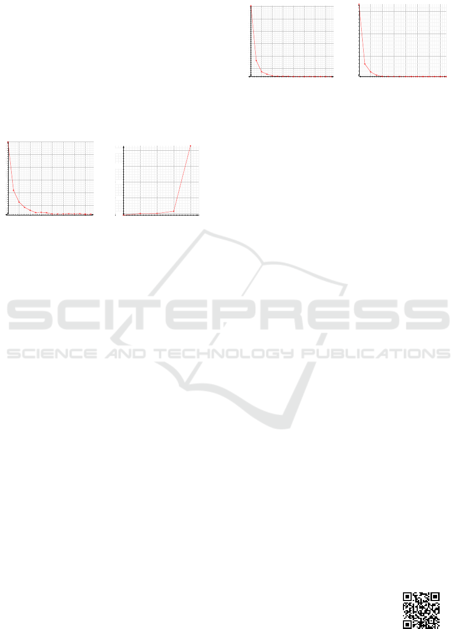
Training in Two Sets of Parameters. This experi-
ment is divided in two stages. In the first stage the ac-
celeration and speed PID parameter tuples are trained.
In the second stage the steering PID parameter tuple
is trained. In stage one the steering PID parameter
tuple needs to be fixed. In order to fix that tuple,
the best PID steering tuple of the first experiment is
taken. This tuple is then inputted to the PID com-
ponent which is responsible for the steering. Fur-
thermore the connection between the Subtraction
component responsible for the steering error and the
ErrorSummation component are dropped. Thus the
steering error will not influence the fitness value. It is
also assured that the steering PID tuple does not bias
the speed and acceleration due to a poor choice of pa-
rameters. To efficiently measure the acceleration and
speed error, the target speed is changed every thirty
seconds alternating between twenty and thirty meters
per second. On the left hand side of Figure 17 the
MSE of the speed and acceleration over the genera-
tions is illustrated. Note that the absolute values of
both experiments cannot be compared due to differ-
ent underlying meta data.
In the second stage of the experiment only the
steering PID parameters are trained. Thus we input
constant parameter tuples to the PID controllers re-
sponsible for the speed and the acceleration. Further-
more the connections between the two Subtraction
components and the ErrorSummation component is
2 4
6
8 10 12 14
200
400
600
800
1,000
1,200
Generation
Average MSE
(a)
2 4
6
8 10 12 14
2
4
6
·10
−3
Generation
Average Steering MSE
(b)
Figure 17: In (a) the MSE of the acceleration and speed
only is shown. In (b) the MSE of the steering is shown.
dropped. Thus only the steering error is evaluated by
the fitness function. On the right hand of Figure 17,
the MSE of the steering PID parameter tuple is de-
picted. In the two stages of the second experiment,
it is proved how simple it is to test different setups
just by dropping connections and providing different
inputs to certain components.
Noise Level Analysis. Other than in the simulator,
it is not possible for a sensor to measure certain phys-
ical values, e.g. the current position, with infinite ac-
curacy. For acceptance testing we make the applica-
tion more realistic by modeling sensor imperfections
using the Additive White Gaussian Noise (AWGN)
model (Cover and Thomas, 2012). Then, a sensor
measurement of the ground truth value X
i
at time step
i is defined as
Y
i
= X
i
+ Z
i
(10)
Z
i
∼ N (0,σ). (11)
Thereby, X
i
is a placeholder for any of the measured
quantities, namely, speed, gas pedal value, steering
angle, yaw angle, the current and the target position.
To filter the noisy sensor signals, low-pass filters are
used. The experiment is executed for five different
noise levels. For each of these noise levels, the PID
parameters were trained for five generations. After
the training, the MSE of the best PID parameter set
for each noise level was measured during one lap with
the respective noise levels. After the fifth noise level
of 5 dB, the car could not be brought under proper
control and crashed, meaning that the maximum ad-
missible noise level was surpassed. In Fig. 16 on the
right hand side the MSE with respect to the noise level
is depicted. Apparently, the system is able to han-
dle sensor imperfections up to a critical noise level
(σ < 3dB). The latter can be found by means of
Fig. 16.
A video of racing car tuning its pa-
rameters is available at:
https://youtu.be/7llpVLklnPY
MODELSWARD 2018 - 6th International Conference on Model-Driven Engineering and Software Development
176

8 CONCLUSIONS
In this paper a novel modeling approach for CPS fol-
lowing the SMARDT methodology was evaluated.
Therefore, a self-driving vehicle controller for driv-
ing on a track in TORCS was developed. Using
formal SysML diagrams and the MontiCAR mod-
eling language it was possible to hierarchically de-
sign the system and evaluate its performance. Novel
language elements such as component and connec-
tor arrays proved to enhance component decoupling
and reuse, e.g., by allowing the evolutional param-
eter tuner to connect to arbitrary many PID compo-
nents. The strong type system supporting units en-
abled efficient component integrity checks. The mod-
ular architecture description enabled the developers
to experiment with many different variants and con-
figurations of the system. Thereby, a suitable control
strategy could be found and evaluated in an efficient
manner. Finally, the models were used to generate a
working system. Hence, it was shown that MontiCAR
is a homogeneous development framework for mod-
eling, verification, testing, and generation of CPS.
ACKNOWLEDGEMENTS
This research was supported by a Grant from the
GIF, the German-Israeli Foundation for Scientific Re-
search and Development, and by the Grant SPP1835
from DFG, the German Research Foundation.
REFERENCES
Accellera SYSTEMS INITIATIVE (2014). Verilog-AMS
Language Reference Manual. Technical Report 2.4.0.
Aravantinos, V., Voss, S., Teufl, S., H
¨
olzl, F., and Sch
¨
atz, B.
(2015). AutoFOCUS 3: Tooling Concepts for Seam-
less, Model-based Development of Embedded Sys-
tems. In ACES-MB.
Ashenden, P. J. (2010). The designer’s guide to VHDL, vol-
ume 3. Morgan Kaufmann.
˚
Astr
¨
om, K. J. and H
¨
agglund, T. (1995). PID controllers:
theory, design, and tuning, volume 2. Isa Research
Triangle Park, NC.
Baheti, R. and Gill, H. (2011). Cyber-physical systems. The
impact of control technology, 12.
Barrett, C., Deters, M., de Moura, L. M., Oliveras, A., and
Stump, A. (2013). 6 Years of SMT-COMP. J. Autom.
Reasoning, 50(3).
Beck, K., Beedle, M., Van Bennekum, A., Cockburn, A.,
Cunningham, W., Fowler, M., Grenning, J., High-
smith, J., Hunt, A., Jeffries, R., et al. (2001). Man-
ifesto for agile software development.
Berger, C. (2016). An Open Continuous Deployment In-
frastructure for a Self-driving Vehicle Ecosystem. In
IFIP International Conference on Open Source Sys-
tems.
Bernhard Wymann, Eric Espi
´
e, C. G. C. D. R. C. and Sum-
ner, A. (2013). TORCS, the open racing car simulator.
Bertram, V., Maoz, S., Ringert, J. O., Rumpe, B., and
von Wenckstern, M. (2017). Case Study on Struc-
tural Views for Component and Connector Models. In
MODELS.
Bertram, V., Roth, A., Rumpe, B., and von Wenckstern, M.
(2016). Extendable Toolchain for Automatic Compat-
ibility Checks. In OCL’16.
Bojarski, M., Del Testa, D., Dworakowski, D., Firner, B.,
Flepp, B., Goyal, P., Jackel, L. D., Monfort, M.,
Muller, U., Zhang, J., et al. (2016). End to end learn-
ing for self-driving cars. Technical report, NVIDIA.
Br
¨
ohl, A.-P. and Dr
¨
oschel, W. (1995). Das V-Modell.
M
¨
unchen, Wien: Oldenburg-Verlag.
Broy, M. and Rausch, A. (2005). Das neue v-modell® xt.
Informatik-Spektrum, 28(3).
Broy, M. and S¸tef
˘
anescu, G. (2001). The algebra of stream
processing functions. Theoretical Computer Science,
258(1-2).
Broy, M. and Stolen, K. (2012). Specification and develop-
ment of interactive systems: focus on streams, inter-
faces, and refinement. Springer Science & Business
Media.
Camacho, E. F. and Alba, C. B. (2013). Model predictive
control. Springer Science & Business Media.
Chen, C., Seff, A., Kornhauser, A., and Xiao, J. (2015).
Deepdriving: Learning affordance for direct percep-
tion in autonomous driving.
Cover, T. M. and Thomas, J. A. (2012). Elements of infor-
mation theory. John Wiley & Sons.
Cramer, E., Kamps, U., and Steland, A. (2008). Grund-
lagen der Wahrscheinlichkeitsrechnung und Statistik.
Springer.
Dautelle, J.-M. and Keil, W. (2010). JSR 275: Units Speci-
fication. Java specification request, RWTH Aachen.
De Moura, L. and Bjørner, N. (2008). Z3: An efficient SMT
solver. In TACAS.
Dormoy, F.-X. (2008). Scade 6: a model based solution for
safety critical software development. In ERTS.
Elmqvist, H., Mattsson, S. E., and Otter, M. (1999).
Modelica-a language for physical system modeling,
visualization and interaction. In CAV.
Friedrich, J., Kuhrmann, M., Sihling, M., and Hammer-
schall, U. (2009). Das v-modell xt. Springer.
Gogolla, M., B
¨
uttner, F., and Richters, M. (2007). USE: A
UML-based specification environment for validating
UML and OCL. Science of Computer Programming,
69(1).
Gray, J. W. (2004). PID Routines for MC68HC11K4 and
MC68HC11N4 Microcontrollers.
Grazioli, F., Kusmenko, E., Roth, A., Rumpe, B., and von
Wenckstern, M. (2017). Simulation Framework for
Executing Component and Connector Models of Self-
Driving Vehicles. In EXE at MODELS.
Model-Based Development of Self-Adaptive Autonomous Vehicles using the SMARDT Methodology
177

Grimm, K. (2003). Software Technology in an Automotive
Company: Major Challenges. In ICSE.
Harel, D. and Rumpe, B. (2004). Meaningful Modeling:
What’s the Semantics of ”Semantics”? IEEE Com-
puter, 37(10).
Kim, J.-S., Kim, J.-H., Park, J.-M., Park, S.-M., Choe, W.-
Y., and Heo, H. (2008). Auto tuning PID controller
based on improved genetic algorithm for reverse os-
mosis plant. World Academy of Science, Engineering
and Technology, 47(2).
Kusmenko, E., Roth, A., Rumpe, B., and von Wenckstern,
M. (2017). Modeling Architectures of Cyber-Physical
Systems. In ECMFA.
Liang, Y.-z. D. C., Wang, Y.-z., and Liu, Y.-f. (2004). The
formal semantics of an UML activity diagram. Jour-
nal of Shanghai University (English Edition).
Liggesmeyer, P. (2009). Software-Qualit
¨
at: Testen,
Analysieren und Verifizieren von Software. Springer
Science & Business Media.
Maoz, S., Mehlan, F., Ringert, J. O., Rumpe, B., and von
Wenckstern, M. (2017). Ocl framework to verify
extra-functional properties in component and connec-
tor models. In ModComp at MODELS.
Maoz, S., Ringert, J. O., and Rumpe, B. (2011). An Oper-
ational Semantics for Activity Diagrams using SMV.
Technical report, RWTH Aachen.
Mathworks Inc. (2016). Simulink User’s Guide. Technical
Report R2016b, MATLAB & SIMULINK.
Matinnejad, R., Nejati, S., and Briand, L. C. (2017). Au-
tomated testing of hybrid Simulink/Stateflow con-
trollers: industrial case studies. In FSE.
Mingsong, C., Xiaokang, Q., and Xuandong, L. (2006).
Automatic test case generation for UML activity di-
agrams. In AST.
Modelica Association (2005). Modelica language specifi-
cation. Link
¨
oping, Sweden.
Montemerlo, M., Becker, J., Bhat, S., Dahlkamp, H., Dol-
gov, D., Ettinger, S., Haehnel, D., Hilden, T., Hoff-
mann, G., Huhnke, B., et al. (2008). Junior: The
stanford entry in the urban challenge. Journal of field
Robotics, 25(9).
National Instruments (1998). BridgeView and LabView: G
Programming Reference Manual. Technical Report
321296B-01.
OMG (2015). OMG Systems Modeling Language (OMG
SysML). Technical Report Version 1.4.
Palmisano, A., Hoops, S., Watson, L. T., Jones, T. C.,
Tyson, J. J., and Shaffer, C. A. (2015). JigCell Run
Manager (JC-RM): a tool for managing large sets of
biochemical model parametrizations. BMC Systems
Biology, 9(1).
Philipps, J., Pretschner, A., Slotosch, O., Aiglstorfer, E.,
Kriebel, S., and Scholl, K. (2003). Model-Based Test
Case Generation for Smart Cards. Electronic Notes in
Theoretical Computer Science, 80(Supplement C).
Pretschner, A., Slotosch, O., Aiglstorfer, E., and Kriebel, S.
(2004). Model-based testing for real. International
Journal on Software Tools for Technology Transfer,
5(2-3).
Rathore, A. and Kumar, M. (2015). Robust Steering Control
of Autonomous Underwater Vehicle: based on PID
Tuning Evolutionary Optimization Technique. Inter-
national Journal of Computer Applications.
Richenhagen, J., Rumpe, B., Schloßer, A., Schulze, C.,
Thissen, K., and von Wenckstern, M. (2016). Test-
driven Semantical Similarity Analysis for Software
Product Line Extraction. In SPLC.
Rumpe, B. (1996). Formale Methodik des Entwurfs verteil-
ter objektorientierter Systeme. Herbert Utz Verlag
Wissenschaft.
Rumpe, B. (2003). Model-Based Testing of Object-
Oriented Systems. In Symposium on Formal Methods
for Components and Objects.
Rumpe, B. (2016). Modeling with UML: Language, Con-
cepts, Methods. Springer International.
Rumpe, B. (2017). Agile Modeling with UML: Code Gen-
eration, Testing, Refactoring. Springer International.
Rumpe, B., Schulze, C., von Wenckstern, M., Ringert, J. O.,
and Manhart, P. (2015). Behavioral Compatibility of
Simulink Models for Product Line Maintenance and
Evolution. In SPLC.
Slicker, J. M. and Loh, R. N. (1996). Design of robust vehi-
cle launch control system. IEEE transactions on con-
trol systems technology, 4(4).
The Institute of Electrical and Electronics Engineers (1988).
Standard VHDL language reference manual. IEEE
Std.
Urmson, C. et al. (2008). Self-driving cars and the urban
challenge. IEEE Intelligent Systems, 23(2).
Utkin, V. (2009). Sliding mode control. CONTROL
SYSTEMS, ROBOTICS AND AUTOMATION–Volume
XIII: Nonlinear, Distributed, and Time Delay Systems-
II.
V-Modell XT (2006). Part 1: Fundamentals of the V-
Modell. Technical report, Federal Government of Ger-
many.
Wei, J., Snider, J. M., Kim, J., Dolan, J. M., Rajkumar,
R., and Litkouhi, B. (2013). Towards a viable au-
tonomous driving research platform. In Intelligent Ve-
hicles Symposium (IV), 2013 IEEE.
Weicker, K. (2007). Evolution
¨
are Algorithmen. Leitf
¨
aden
der Informatik. Vieweg+Teubner Verlag.
Ziegler, J., Bender, P., Schreiber, M., and more (2014).
Making Bertha Drive; An Autonomous Journey on a
Historic Route. IEEE Intelligent Transportation Sys-
tems Magazine, 6(2).
MODELSWARD 2018 - 6th International Conference on Model-Driven Engineering and Software Development
178
