
Diffusion and Disappearance of Traffic Congestion under Steady State in
a Graph Network
Masaru Kaji
1,2
1
Graduate School of Decision Science and Technology, Tokyo Institute of Technology,
2-12-1 Ookayama, Meguro-ku, Tokyo 152-8552, Japan
2
Japan Society for the Promotion of Science,
8 Ichibancho, Kojimachi, Chiyoda-ku, Tokyo, 102-8472, Japan
Keywords:
Traffic Jam, Wave Propagation, Alleviation of Congestion, Steady State, Graph Theory.
Abstract:
Traffic jams on highways or crowds of people in stations during rush hours are social phenomena that have
attracted the attention of many scientists. It is known that the stop-and-go wave is a cluster wave that prop-
agates in a direction opposite to the movement of vehicles or pedestrians. A city consists of many roads and
intersections in the form of a network, and the stop-and-go wave will propagate according to the road network.
Therefore, observations need to be made from a broader perspective to analyze the interconnections between
roads when considering traffic congestion. In this study, we use a graph-based control method and define a
graph-shaped traffic network considering the characteristics of traffic flow. We set the steady state as the ini-
tial condition in the network and create a traffic jam on a certain road intentionally. Following the congestion,
we show the manner in which the traffic congestion wave spreads, and discuss the mechanism in which it
propagates from one road to a connecting road. This also shows the kind of situations in which traffic jams
propagate and diminish; the simulation results correspond to the theoretical value integrated quantitatively.
This will be helpful in solving the traffic congestion problem.
1 INTRODUCTION
Traffic jams in urban areas have been a major prob-
lem for a very long time. We can primarily observe
this phenomenon in stations during rush hours (pedes-
trian dynamics) or on highways (vehicular dynamics)
on a daily basis. Traffic jams cause inefficient flow of
pedestrians or vehicles,and may even lead to a crash
involving several vehicles or a pedestrian crowd dis-
aster. To solve this problem, many researchers have
studied the characteristics of traffic dynamics. For
example, the traffic flow efficiency rapidly decreases
when a traffic jam occurs because the traffic density
is greater than a threshold value for both pedestrian
traffic(Polus et al., 1983; Mori and Tsukaguchi, 1987;
Helbing and Al-Abideen, 2007; Kretz and Schreck-
enberg, 2006) and vehicular traffic (Kerner and Re-
hborn, 1997; Kerner, 1998; Geloliminis and F., 2008;
Daganzo et al., 2011). Moreover, the traffic jam re-
sults in a cluster that consists of some vehicles and
the cluster moves in a direction opposite to the move-
ment of vehicles on the highway (Kerner and Re-
hborn, 1997; Kerner, 1998). This phenomenon is
also confirmed in pedestrian dynamics (Helbing and
Al-Abideen, 2007; Kretz and Schreckenberg, 2006;
Zhang et al., 2012; Jiayue et al., 2014). Pedestrians
or vehicles that are involved in the congestion reduce
their speed and stop. They start to move again when
the vehicle or the pedestrian ahead moves. On the
basis of the series of these movements, scientists call
this wave propagation a stop-and-go wave.
Thus far, most studies on traffic flow have consid-
ered only one subsystem such as a road (Polus et al.,
1983; Mori and Tsukaguchi, 1987; Kerner and Re-
hborn, 1997; Kerner, 1998; Geloliminis and F., 2008;
Daganzo et al., 2011; Zhang et al., 2012), an inter-
section (Lammer and Helbing, 2008; Papageorgiou
et al., 2003), or ajunction (Kernerand Rehborn, 1997;
Kerner, 1998; Papageorgiouet al., 2003). However, in
real-time traffic, paths for pedestrian movement and
roads for vehicles are connected and extend in a net-
work through intersections or junctions. The effect of
the traffic condition on a road is transmitted to the ad-
jacent roads via the joint. Therefore, we need to dis-
cuss the macroscopic system as a composite subsys-
tem. In fact, recently, traffic dynamics has been stud-
ied in terms of a complex network (Geloliminis and
F., 2008; Daganzo et al., 2011; Lammer and Helbing,
186
Kaji, M.
Diffusion and Disappearance of Traffic Congestion under Steady State in a Graph Network.
DOI: 10.5220/0006581701860193
In Proceedings of the 7th International Conference on Operations Research and Enterprise Systems (ICORES 2018), pages 186-193
ISBN: 978-989-758-285-1
Copyright © 2018 by SCITEPRESS – Science and Technology Publications, Lda. All rights reserved

2008; Shen and Gao, 2008; Ezaki et al., 2015; Kaji,
2016; Tao et al., 2016; Sun et al., 2015; Papageorgiou
et al., 2003). Shen and Gao (Shen and Gao, 2008) an-
alyzed the relationship between the dynamical prop-
erties of transportation and the structure network on
a scale-free network. Geloliminis et al. (Gelolimi-
nis and F., 2008) presented a macroscopic fundamen-
tal diagram (MFD) at a city-scale level in Yokohama,
Japan. They suggested that the MFD relating the av-
erage vehicle density and space-mean vehicle flow
in the city exists for the complete network. Ezaki
et al. (Ezaki et al., 2015) assumed a traffic network
and developed a transportation control method con-
sidering traffic characteristics such as those in (Polus
et al., 1983; Mori and Tsukaguchi, 1987; Helbing and
Al-Abideen, 2007; Kretz and Schreckenberg, 2006;
Kerner and Rehborn, 1997; Kerner, 1998; Gelolim-
inis and F., 2008; Daganzo et al., 2011). They also
calculated the transition boundary condition of the
breakdown of the system in the network, and showed
that the theoretical value matched the simulation re-
sult on a certain region. Tao et al. (Tao et al., 2016)
studied the influence of congestion propagation in a
traffic network by using the Cell Transmission Model
(CTM) theory. They then confirmed the congestion
affects both the upstream and downstream regions of
the road through joints such as the intersection.
In this paper, in contrast to (Tao et al., 2016), we
study the effect of a wave cluster of the traffic jam in
a road network more qualitatively and quantitatively,
by using the model of (Ezaki et al., 2015). The cluster
wave will affect another road and we can predict that
the traffic jam propagates to the other adjacent roads
and then finally diminishes. In this case, a new crucial
consideration is analyzing how the traffic jam spreads
and in what kind of situations traffic congestion van-
ishes. It is important to consider the effect of a stop-
and-go wave in a road network for the prediction of
a dynamical traffic jam. Therefore, we study the dy-
namics by considering graph theory and an improved
control simulation method of closing and opening of
inflow (Ezaki et al., 2015). We assume a traffic road
network considering traffic characteristics such as the
free-flow state and the jammed state. Moreover, we
set the steady state as the initial condition and create
a traffic jam by closing a certain road intentionally.
Consequently, we analyze the effect of traffic con-
gestion, discuss diffusion and alleviation of the traf-
fic jam, and discuss qualitatively the conditions under
which the traffic congestion vanishes in the model.
This paper is organized as follows. Section 2 de-
scribes the graph used in this study and the simulation
method. In Section 3, we show the results of this sim-
ulation and interpret them to qualitativelyexplain how
the traffic jam spreads and quantitatively determine
the situations in which traffic congestion vanishes in
the graph. Finally, we state the conclusions and areas
for future research in Section 4.
2 METHOD
To prepare the traffic network, we use graph theory
for analyzing the flow state in digraph. Graph G in
this study consists of a set V
d
of vertices and a set
A
d
of arcs (A
d
⊂ V
d
× V
d
). Note that a vertex and
an arc represent a crossing and a one-way street, re-
spectively. Each arc represents a connection from a
vertex to another vertex so as to not encounter a dead
end. All in-degrees and out-degrees in G have the
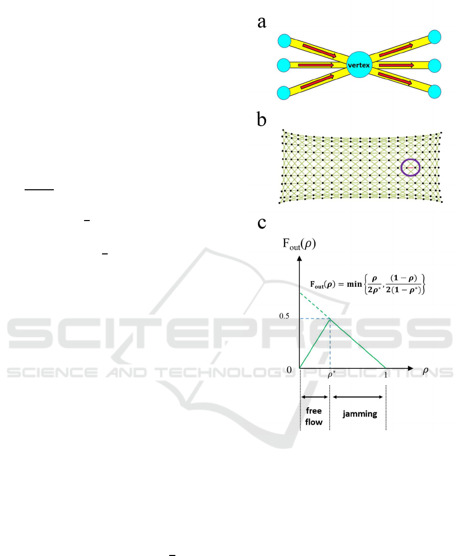
same value, i.e. three, as shown in Fig. 1a. Therefore,
graph G is a cubic directed closed graph. Further-
more, we assume that the number of vertices |G| and
arcs kGk is 200 and 600, respectively. To visualize
the state in G clearly, we draw 10 vertices vertically,
and 30 vertices horizontally. Each arc is connected
from a vertex to the three neighboring vertices on the
right, and the rightmost vertices are joined to the three
leftmost ones. Thereby, we assume that G is periodic
and has a directional structure from left to right. In
addition, we connect the uppermost vertices and the
lowermost vertices to include the effect of the oppo-
site arc. Therefore, the structure of G is Torus and
Fig. 1b is the development elevation of G. Moreover,
we regard a
ij
as an arc connecting vertex i to vertex
j (i 6= j | i, j ∈ V
d
). Every arc includes any number
of objects and the density of the objects in a
ij
at time
step t is ρ
ij
(t). We define the outflow from a
ij
as F
out
(ρ
ij
) (0 ≤ ρ, F
out
≤ 1). The transportation efficiency
is rapidly decreased and a traffic jam occurs when the
pedestrian or vehicle density is over a critical density.
Based on the traffic characteristics, we determine the
value of F
out
as follows:
F
out
(ρ) = min
ρ
2ρ
∗
,
1− ρ
2(1− ρ
∗
)
. (1)
This simple function expresses the free-flow state and
the jammed state (Fig. 1c). In general, vehicles
or pedestrians can move smoothly in the free-flow
state. In the jammed state, on the other hand, the
traffic flow becomes inefficient and there is a possi-
bility that traffic congestion might occur. Note that
Ezaki et al. (Ezaki et al., 2015) assumed that every
vertex included some density instead of every arc and
discussed the interaction between each vertex; how-
ever, we assume that there is some density in each arc
to consider a more realistic situation in the scenario
when vehicles or pedestrians move in the network.
Diffusion and Disappearance of Traffic Congestion under Steady State in a Graph Network
187
When the density in an arc is greater than the thresh-
old ρ
cl
, we prevent inflow into the arc by closing the
entrance of the arc, allowing only outflow from the
arc. Furthermore, a closed arc is opened when the
density of the arc is less than ρ
op
by discharging the
density into another arc. With regards to the inflow
rule, we consider a detouring pattern. In the detour-
ing pattern, the objects flowing from the departure arc
are distributed equally in all open arcs. If all three
destination arcs are closed, the outflow from the arc is
canceled. In addition, the time development of den-
sity on arc a
ij
at t is given by
dρ
ij
(t)
dt
= Q
in
(a
ij
,t) − Q
out
(a
ij
,t)
=
1
3
V
d
∑
h
A
hi
B
ij
F
out
(ρ
hi
(t))
−
1
3
V
d
∑
k
A
jk
B
jk
F
out
(ρ
ij
(t)), (2)
where Q
in
(a
ij
,t) and Q
out
(a
ij
,t) are the total inflow
to a
ij
and outflow from a
ij
, respectively. Note that
the transfer flow depends on conditions at the current
arc and downstream. Moreover, A
ij
is 1 when there
is an arc from vertex i to vertex j (i, j ∈ V
d
, i 6= j),
otherwise A
ij
is 0. Furthermore, B
ij
is 1 or 0 de-
pending on whether a
ij
is opened or closed, respec-
tively. Apart from the detouring pattern, we can also
consider a queuing pattern in which the objects flow-
ing from the departure arc stay there if the arrival arc
is closed. However, the queuing pattern has already
been studied in (Kaji, 2016). We discuss only the case
of the detouring pattern in this study.
We define the vertices and arcs first in our simula-
tion. After that, the initial density at each arc is set as t
= 0. Then, the density in each arc is calculated accord-
ing to the above-mentioned rules. After this calcula-
tion, the density in each arc is updated. Afterwards, t
is updated to (t+dt). The simulation is conducted until
t = 100. In this study, we conduct simulations with dt
= 0.0001. Fig. 2 shows the flowchart in this simula-
tion. We set ρ
cl
= 0.75, and ρ
∗
= 0.5 for simplicity.
In this simulation, we assume that every arc in G
is uniformly set with the average density
ρ by the ini-
tial condition, and the amount of inflow is the same as
the amount of outflow, i.e., the initial flow in G is in a
steady state. Then, we generate a traffic jam in an arc
intentionally in graph G at t = 0. We set the density
in the arc, located on the right center in G in Fig.1b,
as ρ
cl
, and we set the state of the arc as closed. In
this way, we can analyze the effect of this on the sur-
rounding arcs.
Figure 1: (a) Diagram of a vertex with three arcs connected
from and three arcs connected to other vertices. (b) The de-
veloped elevation of G. The uppermost vertices are the same
as the lowermost vertices. In the same way, the rightmost
vertices are the same as the leftmost vertices. Therefore,
the structure of G is Torus and the objects move from left to
right. In this simulation, we generate a traffic jam intention-
ally in an arc surrounded by the purple circle (the red arc).
(c) Function F
out
(ρ) versus the density ρ.
3 RESULTS AND DISCUSSION
3.1 State of the Graph after the
Occurrence of Traffic Congestion
When viewing the state of G at t = 100 and ρ
op
=
0.60, there are roughly three phases, i.e., the free-flow
ICORES 2018 - 7th International Conference on Operations Research and Enterprise Systems
188
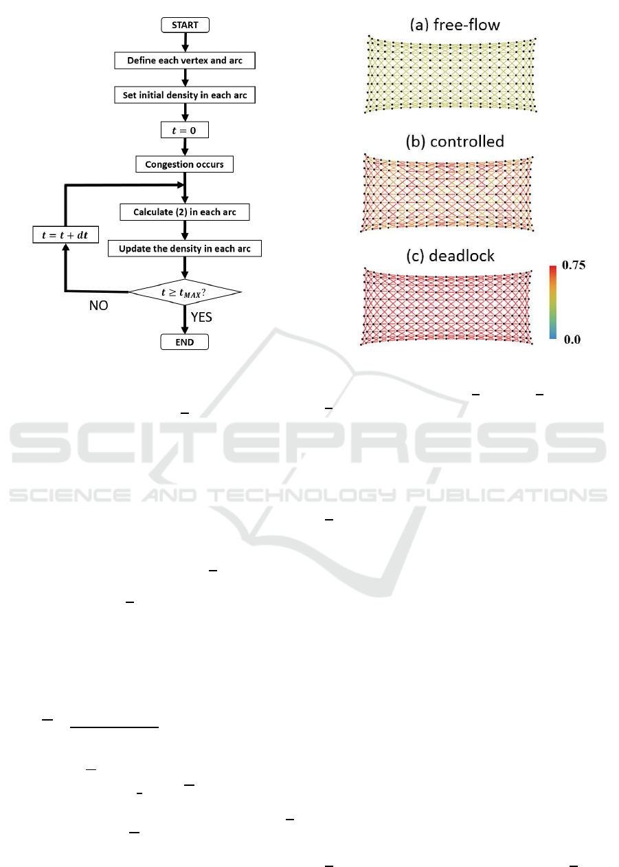
Figure 2: Flowchart used in this study.
phase, the controlled phase, and the deadlock phase,
which are obtained by changing
ρ (Fig. 3). Note that
the red arcs in Fig. 3 express the closed state. In the
free-flow state, traffic congestion is solved immedi-
ately and the state in G returns to the original steady
state (Fig. 3a). In the case of the controlled phase,
some congestion continues to exist locally in G and
moves from an arc to another arc (Fig. 3b). On the
other hand, in the deadlock phase, all arcs in G are
closed and the flow in G breaks down because of the
congestion generated at t = 0 (Fig. 3c).
We show the phase diagram in the
ρ and ρ
op
plane
at t = 100 in Fig. 4a. From this figure, we can see that
the phase depends on
ρ and ρ
op
. The area ∗ in Fig.
4a is a kind of controlled phase. In this area, only the
arc in which congestion was generated intentionally
repeats the steps of closed and opened states as ρ
op
is
relatively large and the flow is always inefficient even
if the arc is opened. Furthermore, we calculated the
average flow rate in G. We defined the average flow
rate as
Q =
∑
V
d
i
∑
V
d
j
A
ij
Q
out
(a
ij
)
kGk
. The MFD is shown in
Fig. 4b. Figs. 4a and 4b show that efficient flow is
achieved in the free-flow state, and also show the av-
erage flow rate
Q in the graph along with the value of
function (1) when ρ
∗
=
1
2
. Here
Q rapidly decreases
just as the phase changes from the free-flow phase to
the controlled phase, and is gradually reduced as
ρ
increases. Eventually, Q is 0 in the deadlock phase.
Note that the flow rate in ∗ achieves efficient flow be-
cause there is only one closed arc.
Figure 3: States in the graph in the case of the free-flow
phase, the controlled phase, and the deadlock phase where
ρ
op
= 0.60, at t = 100, and (a)
ρ = 0.35, (b) ρ = 0.60, and (c)
ρ = 0.75. The value of density matches the color bar.
3.2 How the Traffic Congestion Spreads
We analyzed the controlled phase in detail. In this
phase, we can divide the movement of the congestion
into four patterns by changing the parameters ρ
op
and
ρ. Fig. 5 shows a snapshot for each of these simu-
lations. In Fig. 5a, the congestion in the arc propa-
gates in a direction opposite to the movement of ob-
jects (to the left) as a recession wave and crosswise
(to the vertical). The width of the wave gradually in-
creases and the wave transforms into a large one. In
Fig. 5b, the movement of the wave is the same as
that of the wave in Fig. 5a in the early stage. How-
ever, the rear part of the congestion wave (right side)
is stagnant in some arcs. The speed of the nose of
the wave gradually decreases. In Fig. 5c, the conges-
tion arc affects not only the direction opposite to the
movement of the objects, but also the direction of the
movement of the objects (the traveling wave). After a
while, the traveling wave collides with the recession
wave, forms some new waves, and moves to the left
in the graph. In Fig. 5d, on the other hand, the move-
ment of the wave exhibits the same behavior as that
in Fig. 5c in an early stage. After that, the conges-
tion wave does not grow and each congestion wave
continues to move finely in the graph. In general, we
confirmed the phenomenon in Figs 5a and 5b when
ρ is less than 0.5 (more generally speaking, ρ ≤ ρ
∗
).
Diffusion and Disappearance of Traffic Congestion under Steady State in a Graph Network
189
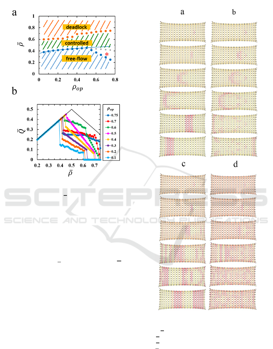
Figure 4: (a) Phase diagram for this simulation. The ver-
tical and the horizontal axes represent the open arc density
ρ
op
and the average density
ρ, respectively, at t = 100 and
ρ
∗
= 0.5. The blue circles indicate the border between the
free-flow phase and the controlled phase. The orange cir-
cles indicate the border between the controlled phase and
the deadlock phase. The area within the star surrounding
the blue circles and the gray circles show the phase in which
the only arc where congestion was generated intentionally
repeats the steps from being in the closed state to the open
state and vice versa. The blue solid line is the theoretical
value of the function (7). (b) Macroscopic fundamental dia-
gram of Fig. 4a. The vertical and the horizontal axes denote
the initial average density
ρ and the average flow rate Q, re-
spectively. The solid line corresponds to function (1).
Otherwise, the phenomenon shown in Figs. 5c and
5d occurs. Moreover, the simulation result shown in
Fig. 5a is found to hold when ρ
op
is relatively small.
The result gradually has the nature of Fig. 5b from
when ρ
op
is approximately 0.55. On the other hand,
the phenomenon in Fig. 5c begins to move into that
of Fig. 5d when ρ
op
is about 0.58. Both the recession
wave and the traveling wave propagate faster as the
initial average density increases.
Next, we discuss the mechanisms of the phe-
nomenon in which the congestion wave moves in a
direction opposite to the movement of objects as ob-
served in Figs. 5a, 5b, 5c, and 5d. When traffic con-
gestion occurs in an arc, the outflow from the three
arcs located on the next congestion arc to the right is
Figure 5: Snapshots of the wave propagation by the four
patterns in the controlled phase. The conditions are: (a) ρ
op
= 0.40,
ρ = 0.45, at t = 3, 5, 10, 15, 25, and 45; (b) ρ
op
=
0.60,
ρ = 0.45, at t = 9, 15, 20, 30, 40, and 50; (c) ρ
op
=
0.40,
ρ = 0.55, at t = 1, 2, 3, 5, 10, and 20; and (d) ρ
op
=
0.60,
ρ = 0.60, at t = 1, 2, 3, 5, 10, and 20.
limited. Despite this, the inflow to these three arcs
does not change. Hence, the density of these arcs
gradually increases. As a result, these three arcs fall
into a state of congestion. This event successively
ICORES 2018 - 7th International Conference on Operations Research and Enterprise Systems
190

propagates in a direction opposite to the movement
of the recession wave.
In the case of the phenomenon in which the rear
part of the congestion wave (right side) is stagnant in
some arcs in Figs 5b and 5d, the congestion arc cannot
recover from the jammed state to the free-flow state
easily because the value of ρ
op
is relatively large and
the flow soon becomes inefficient, even if the arc re-
turns from the closed state to the open state. Thereby,
the arc is no longer in the inefficient flow state and
alternates between the closed and the open states.
When the traveling wave occurs as shown in Figs
5c and 5d, the outflow from the congestion arc is rela-
tively small compared with the outflow from the three
arcs, which are located on the right side of the con-
gestion arc. Therefore, the density in these arcs grad-
ually decreases, and the outflow from these arcs in-
creases. Thereby, the inflow of the following arcs on
the right increases and so does the density of these
arcs. Finally, these arcs transit from the inefficient
flow state to the congestion state. By repeating the
mechanism in a direction to the right, the wave prop-
agates to the right. This phenomenon occurs when
ρ >
1
2
(speaking more generally,
ρ > ρ
∗
). However,
the phenomenon will not occur intuitively in a real-
time vehicle or pedestrian dynamics because the traf-
fic congestion affects the vehicles or pedestrians at the
rear when the general stop-and-go wave propagates
backward.
3.3 Kinds of Situations in which the
Traffic Congestion Vanishes
We now discuss the phase transition to determine
whether a congestion arc affects the arcs at the back
(to the left in this simulation) or not. In this paper,
we discuss only ρ
op
≤
1
2
(or ρ
op
≤ ρ
∗
). When an arc
is congested with traffic (the closed state), we need to
consider the critical density ρ’, which is the density of
the arcs next to the congestion arc on the right when
the congestion arc recovers from the closed state to
the open state. That is, the congestion arc affects the
following arcs if the time T
ρ→ρ
′
, which is required for
increasing the density of the arcs from
ρ to the critical
density ρ’, is greater than the time T
ρ
cl
→ρ
op
required
for recovering from the closed state to the open state.
We can change equation (2) as dt =
dρ
∆Q
, i.e., the nor-
malization constant, T
ρ
cl
→ρ
op
can be presented as
T
ρ
cl
→ρ
op
=
Z
ρ
op
ρ
cl
dρ
−Q
out
=
Z 1
2
ρ
op
dρ
ρ
+
Z
ρ
cl
1
2
dρ
1− ρ
= log
1
4(1− ρ
cl
)ρ
op
. (3)
Roughly speaking, the congestion cluster does not
propagate unless the inflow in an arc is greater than
the outflow on the road. Therefore, when T
ρ
cl
→ρ
op
= T
ρ→ρ
′
, the boundary condition for whether a con-
gested road affects the adjacent rear roads or not, can
be presented as
ρ
′
= 1−
ρ. (4)
Here, we assume that the relation
ρ <
1
2
always holds.
Intuitively, it is true because of the simulation results
in Fig. 4a. Next, from (2), assuming the arc is in the
steady state, the time development of the density on
an arc, which is located on the congestion arc at the
back, becomes
dρ
dt
= Q
in
− Q
out
=
ρ−
2
3
min{ρ, 1− ρ}, (5)
where Q
in
is constant
ρ. When ρ
op
≤
1
2
, T
ρ→ρ
′
is
given by
T
ρ→ρ
′
=
Z
ρ
′
ρ
dρ
Q
in
− Q
out
=
Z
1
2
ρ
dρ
ρ−
2
3
ρ
+
Z
ρ
′
1
2
dρ
ρ−
2
3
(1− ρ)
= 2
Z 1
2
ρ
dρ
ρ−
2
3
ρ
(6)
= 3log
ρ
3ρ− 1
, (7)
where (6) is derived from the symmetry that ρ
′
= 1 -
ρ as we regard ρ=
1
2
as a median Assuming that the
boundary density
ρ
trans
is the average density ρ when
T
ρ→ρ
′
= T
ρ
cl
→ρ
op
, we consider the boundary condition
(4) and derive from (3) and (7)
Diffusion and Disappearance of Traffic Congestion under Steady State in a Graph Network
191
ρ
trans
=
1
4(1−ρ
cl
)ρ
op
1
3
3
1
4(1−ρ
cl
)ρ
op
1
3
− 1
. (8)
The theoretical values of (8) match the simulation re-
sults shown in Fig. 4a.
Moreover, we further generalize (8). When ρ
∗
is a
variable, i.e., when F
out
satisfies function (1), we can
rewrite (3) as
T
ρ
cl
→ρ
op
= 2log
(
ρ
∗
ρ
op
ρ
∗
1− ρ
∗
1− ρ
cl
(1−ρ
∗
)
)
. (9)
Furthermore, we derive the boundary condition from
(4)
ρ
′
= 1−
1− ρ
∗
ρ
∗
ρ. (10)
Assume that the relations
ρ < ρ
∗
and Q
in
=
ρ
2ρ
∗
are al-
ways practical, we can derive from (5) and (10) when
ρ
op
< ρ
∗
in the relation
T
ρ→ρ
′
=
Z
ρ
∗
ρ
dρ
ρ
2ρ
∗
−
2
3
ρ
2ρ
∗
+
Z
ρ
′
ρ
∗
dρ
ρ
2ρ
∗
−
2
3
1−ρ
2(1−ρ
∗
)
= 3log
ρ
3ρ− 2ρ
∗
. (11)
With (9) and (11), we finally obtain
ρ
trans
=
2ρ
∗
ρ
∗
ρ
op
2
3
ρ
∗
1−ρ
∗
1−ρ
cl
2
3
(1−ρ
∗
)
3
ρ
∗
ρ
op
2
3
ρ
∗
1−ρ
∗
1−ρ
cl
2
3
(1−ρ
∗
)
− 1
. (12)
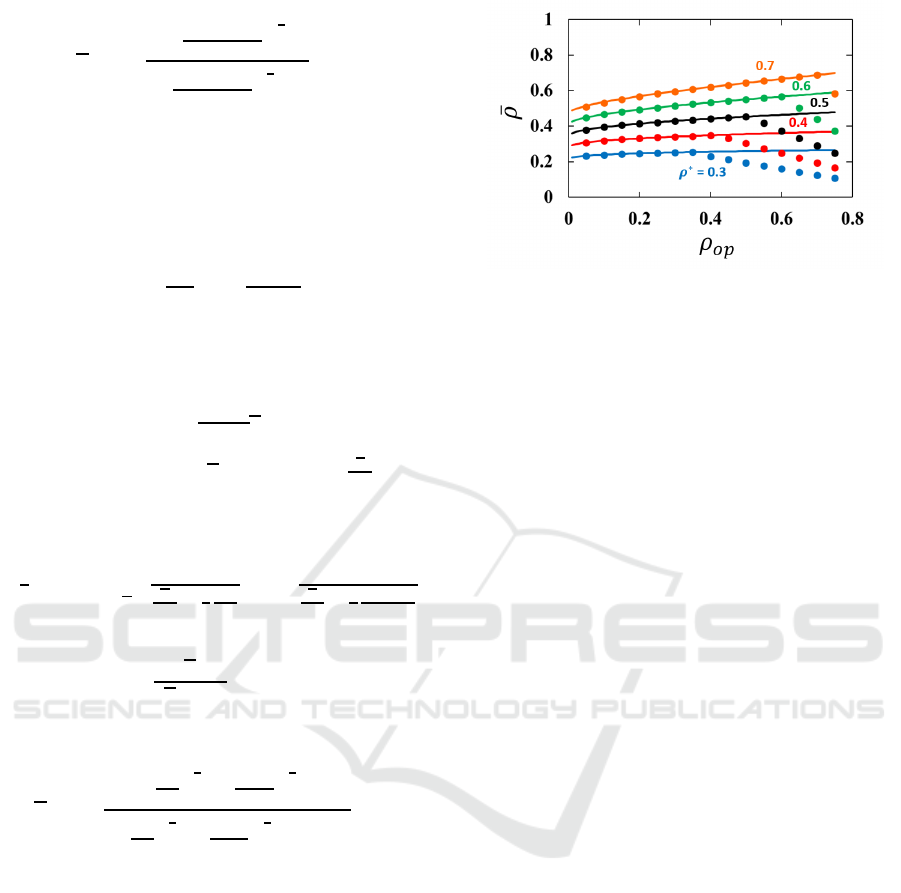
Fig. 6 shows the theoretical values of function (12)
and the simulation results in each ρ
∗
where ρ
cl
= 0.75,
and each theoretical value and the value from the sim-
ulation matches when ρ
op
≤ ρ
∗
.
4 CONCLUSIONS AND FUTURE
RESEARCH
In this paper, we assumed the traffic network to be
a cubic directed closed graph considering the traf-
fic characteristics such as the free-flow state and the
jammed state. Moreover, we have defined the con-
trol method using the closed and open states of in-
flow. We have set the steady state as the initial con-
dition and generated a traffic jam by closing a cer-
tain arc intentionally at a certain time. As a result,
Figure 6: Contour lines between the free-flow phase and the
controlled phase where ρ
cl
= 0.75. The solid lines denote
the theoretical values of function (8) and the dots denote
the simulation results where ρ
cl
= 0.75, ρ
∗
is 0.3 (blue), 0.4
(red), 0.5 (black), 0.6 (green), and 0.7 (orange). Note that
the black dots and line in this figure correspond to the blue
dots and the blue line in Fig. 4a.
there arose three traffic phase patterns in the graph,
i.e., the free-flow phase, the controlled phase, and the
deadlock phase. We have obtained the phase diagram
and found that the phase condition depends on the
open state density of the arc and the initial average
density in the graph. Furthermore, in the controlled
phase, we have confirmed that the congestion move-
ment contains three patterns; the recession wave pat-
tern, the traveling wave pattern, and the stagnation
pattern, formed by changing the opened density and
the initial average density. In addition, we have dis-
cussed the quantitativeassessment related to the effect
of the congestion arc on the other adjacent arcs, i.e.,
the boundary condition between the free-flow phase
and the controlled phase. As a consequence, the theo-
retical value partially corresponded to the simulation
result in the phase diagram. This theory will help us
arriveat the solution of the traffic congestion problem.
However, we could not show the theoretical value
in certain regions. It is necessary to discuss the re-
maining portions for more exact prediction. In addi-
tion, qualitatively discussing the flow condition in the
unsteady state and the inequality distribution rule in
a more realistic traffic network remain unsolved chal-
lenges. Furthermore, this model will be more real-
istic model by changing from the deterministic to the
stochastic. We also need to confirm whether the simu-
lation and theoretical values match the real-time traf-
fic phenomenon. Finally, by developing the model
which can forecast the traffic jam in a road network,
we will be able to apply to the operations research
model such as the time-dependent shortest path prob-
lem in urban network (Cooke and Halsey, 1966; Sun
et al., 2017).
ICORES 2018 - 7th International Conference on Operations Research and Enterprise Systems
192

ACKNOWLEDGEMENTS
This work was supported by a Grant-in-Aid for JSPS
Research Fellows Grant Number 16J03284. Further-
more, I appreciate the feedback offered by my super-
visor, Takehiro Inohara. I also would like to thank
Editage (www.editage.jp) for English language edit-
ing.
REFERENCES
Cooke, K. and Halsey, E. (1966). The shortest route
through a network with time-dependent internodal
transit times. 14(3):493–498.
Daganzo, C. F., Gayah, V. V., and Gonzales, E. J.
(2011). Macroscopic relations of urban traffic vari-
ables: Bifurcations, multivaluedness and instabil-
ity. Transportation Research Part B: Methodological,
45(1):278–288.
Ezaki, T., Nishi, R., and Nishinari, K. (2015). Tam-
ing macroscopic jamming in transportation networks.
Journal of Statistical Mechanics: Theory and Experi-
ment, 2015(6):P06013.
Geloliminis, N. and F., D. C. (2008). Existence of urban-
scale macroscopic fundamental diagrams: Some ex-
perimental findings. Transportation Research Part B:
Methodological, 42(9):759–770.
Helbing, D., J. A. and Al-Abideen, H. Z. (2007). Dynam-
ics of crowd disasters: An empirical study. Physical
review E, 75(4):046109.
Jiayue, W., Wenguo, W., and Xiaole, Z. (2014). Compar-
ison of turbulent pedestrian behaviors between mina
and love parade. In Proceedings of the 2014 Interna-
tional Symposium on Safety Science and Technology,
volume 84, pages 708–714.
Kaji, M. (2016). Analysis of propagation of traffic jam un-
der steady flow (in japanese). In Proceedings of the
22th Symposium on Traffic Flow and Self-Driven Par-
ticles, pages 65–68.
Kerner, B. S. (1998). Experimental features of self-
organization in traffic flow. Physical Review Letters,
81(17):3797.
Kerner, B. S. and Rehborn, H. (1997). Experimental prop-
erties of phase transitions in traffic flow. Physical Re-
view Letters, 79(20):4030.
Kretz, T., G. A. and Schreckenberg, M. (2006). Experi-
mental study of pedestrian flow through a bottleneck.
Journal of Statistical Mechanics: Theory and Experi-
ment, 2006(10):P10014.
Lammer, S. and Helbing, D. (2008). Self-control of traffic
lights and vehicle flows in urban road networks. Jour-
nal of Statistical Mechanics: Theory and Experiment,
2008(04):P04019.
Mori, M. and Tsukaguchi, H. (1987). A new method for
evaluation of level of service in pedestrian facilities.
Transportation Research Part A: General, 21(3):223–
2346.
Papageorgiou, M., Diakaki, C., Dinopoulou, V., Kotsialos,
A., and Wang, Y. (2003). Review of road traffic con-
trol strategies. In Proceedings of the IEEE, volume 91,
pages 2043–2067.
Polus, A., Schofer, J., and Ushpiz, A. (1983). Pedestrian
flow and level of service. Journal of Transportation
Engineering, 109(1):46–56.
Shen, B. and Gao, Z. Y. (2008). Dynamical properties of
tranportation on complex networks. Physica A: Sta-
tistical Mechanics and is Applications, 387(5):1352–
1360.
Sun, L., Liu, L., Xu, Z., Jie, Y., Wei, D., and Wang, P.
(2015). Locating inefficient links in a large-scale
transportation network. Physica A: Statistical Me-
chanics and is Applications, 419:537–545.
Sun, Y., Yu, X., Bie, R., and Song, H. (2017). Discov-
ering time-dependent shortest path on traffic graph for
drivers towards green driving. Journal of Network and
Computer Applications, 83:204–212.
Tao, R., Xi, Y., and Li, D. (2016). Simulation analysis on ur-
ban traffic congestion propagation based on complex
network. In Proceedings of the IEEE Service Opera-
tions and Logistics, and Informatics 2016, pages 217–
222.
Zhang, X. L., Weng, W. G., and Yuan, H. Y. (2012). Empir-
ical study of crowd behavior during a real mass event.
Journal of Statistical Mechanics: Theory and Experi-
ment, 2012(8):P08012.
Diffusion and Disappearance of Traffic Congestion under Steady State in a Graph Network
193
