Simulation-based Optimization of Camera Placement in the Context of

Industrial Pose Estimation

Troels B. Jørgensen

, Thorbjørn M. Iversen

, Anders P. Lindvig

, Christian Schlette

, Dirk Kraft

Thiusius R. Savarimuthu

, J

urgen Roßmann

and Norbert Kr

uger

Mærsk McKinney Møller Institute, University of Southern Denmark, 5230, Odense M, Denmark

Institute for Man-Machine Interaction, RWTH Aachen University, 52074, Aachen, Germany

Keywords:

Pose Estimation, Simulation, Optimization.

Abstract:

In this paper, we optimize the placement of a camera in simulation in order to achieve a high success rate for

a pose estimation problem. This is achieved by simulating 2D images from a stereo camera in a virtual scene.

The stereo images are then used to generate 3D point clouds based on two different methods, namely a single

shot stereo matching approach and a multi shot approach using phase shift patterns. After a point cloud is

generated, we use a RANSAC-based pose estimation algorithm, which relies on feature matching of local 3D

descriptors.

The object we pose estimate is a tray containing items to be grasped by a robot. The pose estimation is done

for different positions of the tray and with different item conﬁguration in the tray, in order to determine the

success rate of the pose estimation algorithm for a speciﬁc camera placement. Then the camera placement

is varied according to different optimization algorithms in order to maximize the success rate. Finally, we

evaluate the simulation in a real world scene, to determine whether the optimal camera position found in

simulation matches the real scenario.

1 INTRODUCTION

When designing vision-based solutions for industrial

systems, the placement of the vision sensor is rarely

investigated in detail. Usually, it is simply placed

where there are space and no obvious occlusion. This

is a suboptimal choice and in some cases it can have

a signiﬁcant impact on the overall success rate of an

industrial system. In this paper, we investigate the ca-

mera placement using a simulation framework to opti-

mize the success rate of a pose estimation application.

There are many advantages of relying on simula-

tion. One is that the basic algorithm can be written

and tested before the actual setup is built. Tests on

real platforms require physical re-arrangements and

re-calibration as well as the performance of many tri-

als where pose estimates need to be manually evalua-

ted in terms of their correctness. Transferring this op-

timization to simulation allows for doing these tests

with simple re-arrangement in simulation with au-

tomated calibration and automated comparison with

ground truth data. Furthermore, it is feasible to do

substantially more experiments, since the only cost is

computation time. This even allows for applying gra-

dient decent like methods to operate on an objective

function instead of unsystematic trial and error on real

platforms. Hence by transferring this process to si-

mulation, set-up times of vision based robot solutions

can be signiﬁcantly reduced.

Researchers have shown that it is these costs in

the set-up of robot assembly processes, that make it

hard to arrive at commercially viable robot solutions

for small batch size production, which is in particu-

lar relevant for SMEs (Kr

uger et al., 2014). However,

photo-realistic rendering is a difﬁcult and computati-

onally expensive task. Therefore, we focus on simpler

and more computationally feasible rendering approa-

ches from the robotic simulation framework VERO-

SIM. Since the images are imperfect, we evaluate the

solutions in the real world as well to show the validity

of the approach.

Simulation-based investigation of robotic soluti-

ons using general purpose simulation frameworks is

an expanding ﬁeld. For example, the eRobotics met-

hodology provides a development platform for robo-

ticists to exchange ideas and to collaborate with ex-

perts from other disciplines (Schluse et al., 2013).

eRobotics aims at providing comprehensive digital

524

Jørgensen, T., Iversen, T., Lindvig, A., Schlette, C., Kraft, D., Savarimuthu, T., Rossmann, J. and Krüger, N.

Simulation-based Optimization of Camera Placement in the Context of Industrial Pose Estimation.

DOI: 10.5220/0006553005240533

In Proceedings of the 13th International Joint Conference on Computer Vision, Imaging and Computer Graphics Theory and Applications (VISIGRAPP 2018) - Volume 5: VISAPP, pages

524-533

ISBN: 978-989-758-290-5

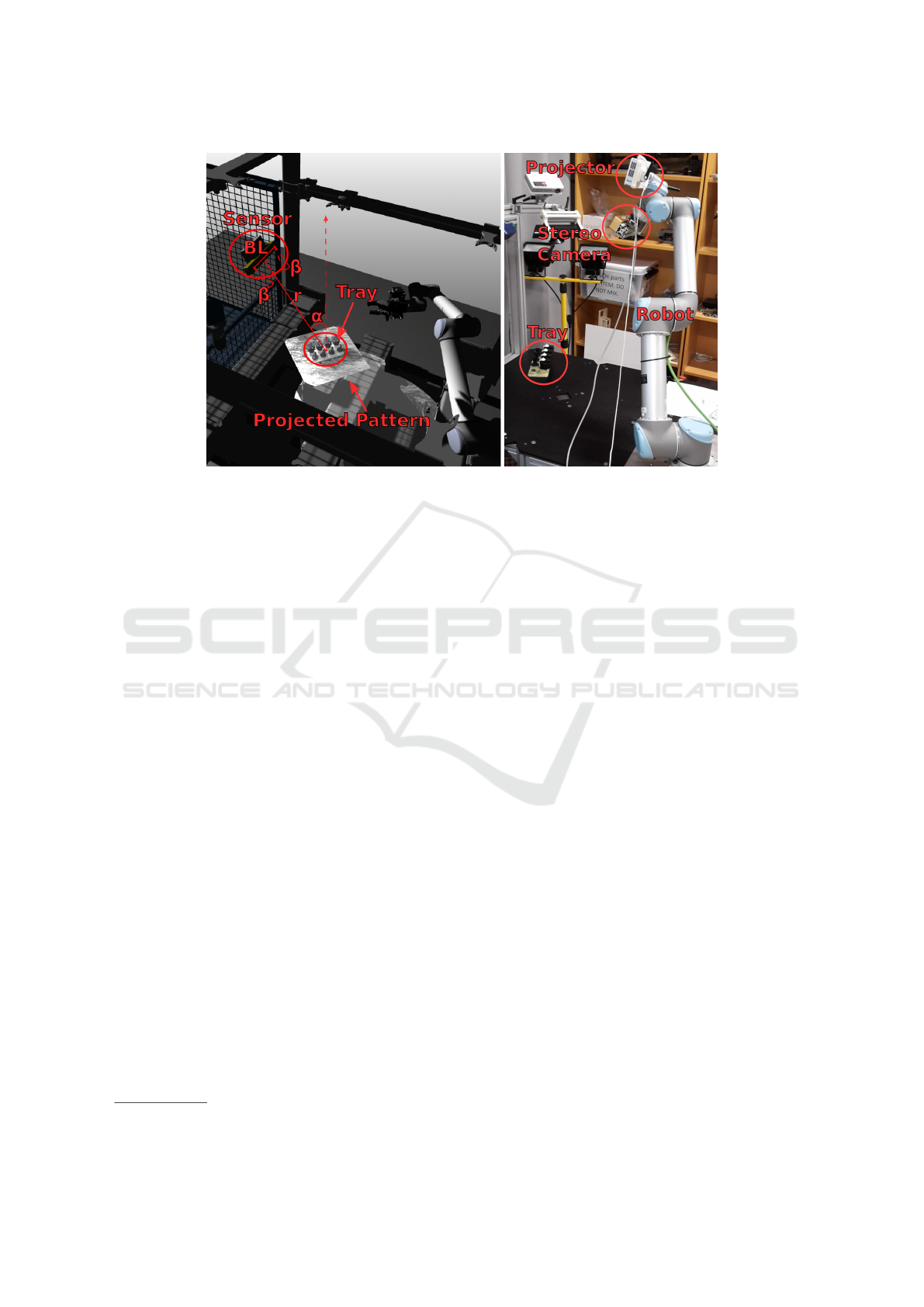
Figure 1: The pose estimation scene. Left) The scene in simulation along with the most important parameters for the sensor

placement. BL is the base-line, β is the vergence, α is the polar angle and r is the radial distance. Right) The real world setup

used for evaluating the realism of the simulated results.

models of complex technical systems and their inte-

raction with prospective working environments in or-

der to design, program, control and optimize them

in 3D simulation before commissioning the real sy-

stem. In this paper, we utilize the eRobotics frame-

work VEROSIM



for simulating the system

, such

that the approach can be easily integrated into a more

complex industrial system.

Utilizing the simulation framework, we investi-

gate whether 3D simulation-based optimization can

be used to improve the pose estimation success rate

of a test case. The case addressed in this paper is a

pose estimation problem, where a tray containing a

random set of items has to be detected. The task is il-

lustrated in Figure 1 and the parameters we optimize

are the placement of the sensor. In Figure 1, it can

be seen that the tray is bright compared to the dark

items placed in it. This further complicates the task

when relying on structured light, since the reﬂective

properties are quite different for the two materials.

The goal of the paper is not to ﬁnd a single set

of parameters that work well for every problem, but

rather to investigate a simulation-based approach for

determining case speciﬁc parameters for a given task.

Therefore, we apply the method to two different trays

and show the performance for both cases.

To solve the pose estimation problem, we start by

generating a point cloud using a stereo camera and

a projector. We then use RANSAC in combination

with point cloud based feature matching to determine

a likely pose of the tray. Here, the model of the tray

see http://www.verosim-solutions.com/en/

used during pose estimation is based on multiple view

points of the tray and multiple combinations of items

in the tray.

The main contributions of the paper are the follo-

wing:

• By computing comprehensively an objective

function for pose estimation in a simulated robot-

vision set-up in a relevant parameter range of ca-

mera placements, we demonstrated that the ca-

mera placement plays an important role for the

success rate of a pose estimation algorithm.

• By brute force computation of pose estimation

quality, we were able to determine a good camera

placement in terms of the polar angle and the ra-

dial distance for the given task.

• By optimizing the objective function by means

of the numeric optimization algorithm RBFopt

(Costa and Nannicini, 2015), we were able to op-

timize additional parameters namely the baseline

and vergence. This resulted in higher success ra-

tes compared to simply optimizing the polar angle

and radial distance with brute force optimization.

• By comparing the results achieved in simulation

and on a real set-up, we show that camera place-

ments with high success rates in simulation mat-

ched camera placements with high success rates in

the real world. Furthermore, we evaluated the full

brute force optimization in simulation and in the

real world, here we show that the pose-estimation

success rate is similar in simulation and in the real

world.

Simulation-based Optimization of Camera Placement in the Context of Industrial Pose Estimation

525

The paper is structured as follows. In Section 2,

we discuss related work with regard to image simula-

tion, pose estimation and optimization. In Section 3,

we introduce the pose estimation pipeline and dis-

cuss the free parameters and the quality metrics. In

Section 4, we discuss the simulation of images and

the two stereo-based approaches used to generate the

point clouds. In Section 5, we discuss the pose es-

timation algorithm in more detail. In Section 6 and

7, we show the optimization results and evaluate the

realism of the simulation results based on real world

trials. Lastly, we conclude on the work and discuss

future extensions in Section 8.

2 RELATED WORK

This paper addresses simulation-based optimization

of camera placements. Several researchers have ad-

dressed similar problems, e.g. (Mavrinac et al., 2015)

where an active triangulation 3D inspection system

is conﬁgured using model-based optimization. The

critical system parameters are optimized using parti-

cle swarm optimization. Another noteworthy article

is presented by (Kouteck

y et al., 2015), where the op-

timal position of an active light scanner is determined

for the reconstruction of highly reﬂective objects. To

improve the realism of the simulated scans in the opti-

mization, the reﬂective properties of the object mate-

rial is empirically determined prior to the simulation.

For an excellent survey of related literature refer to

(Chen et al., 2011).

In this work, we address simulation-based optimi-

zation of camera placement, in order to maximize the

success rate of a pose estimation application. Because

of this both the geometry of the object and a rough

model of the 3D reconstruction method are important.

But we claim that highly realistic simulated images

are not required for this type of pose estimation, un-

like (Kouteck

y et al., 2015), thus we have focused on

simulations that are easy to setup and model, and real

world evaluations indicating that the optimal sensor

placement in simulation is also good in the real world

(see Section 7). Furthermore, we include several ty-

pes of uncertainties from the real world in the simu-

lation, such as background illumination, to ensure the

camera placement is robust to the most common vari-

ations.

The remainder of this section is split into the three

main topics of the paper, namely simulation or rende-

ring of 2D images, pose estimation in 3D and nume-

ric optimization. In the simulation part, we focus on

relatively fast rendering methods with application to

the robotics domain. In the pose estimation section,

we focus on pose estimation based on 3D point cloud

data. In the optimization section, we focus on robust

optimization methods with applications to simulation-

based optimization.

2.1 Simulation and Rendering of 2D

images

Synthetic images have been used in the literature for

various different tasks, e.g. training (Rozantsev et al.,

2015), uncertainty analysis (Dong et al., 2014), ana-

lysis of visual features (Takei et al., 2014) and off-line

programming (Nilsson et al., 2009).

In order to use synthetic images in the context of

computer vision, it is crucial that the images are suf-

ﬁciently realistic such that the computer vision algo-

rithms show similar behavior for the real and synthe-

tic images. However, when rendering synthetic ima-

ges a trade off must be made between realism and ren-

dering speed.

In work presented by (Medeiros et al., 2014),

structured light scanners are benchmarked in simu-

lation using highly realistic synthetic images. These

images are generated using ray tracing which mi-

mics the physical properties of light rays. Physically-

based rendering is however a time consuming techni-

que which makes it unattractive in an optimization

framework, where convergence requires many itera-

tions and thus the generation of many images.

In work presented by (Irgenfried et al., 2011), the

trade off between speed and realism have been hand-

led by developing a system, which allows for both real

time rasterization-based renderings with low realism

or slower ray tracing-based renderings with a high de-

gree of realism.

In work presented by (Rossmann et al., 2012), a

compromise between realism and rendering speed is

made by combining real time rasterization techniques

with advanced lighting and noise modeling. They also

document a test setup which is used to verify that the

generated images actually resembles the real world

images. We have opted for this last approach since

it allows us to incorporate high quality synthetic ima-

ges in a state-of-the-art optimization procedure.

2.2 Pose Estimation

Pose estimation of 3D objects is a common task in ro-

botics (Aldoma et al., 2012), (Papazov and Burschka,

2010) and (Großmann et al., 2015). But in this work,

we focus on the task of pose estimating a tray, con-

taining a random subset of items. In order to achieve

pose estimation with a high success rate, it is neces-

sary to implement a pose estimation strategy that is

VISAPP 2018 - International Conference on Computer Vision Theory and Applications

526

not substantially affected by missing items. This task

is less explored, but a somewhat similar task arises

in articulated pose estimation of humans, where it is

also necessary to estimate the pose based on various

subcomponents of the entire object. Various appro-

aches exist for solving this problem, such as data-

base lookups to determine similar conﬁgurations (Ye

et al., 2011), and ICP reﬁnement based on splitting

the human into sub-components and ﬁne tuning these

(Knoop et al., 2006).

Since the items, in our pose estimation case, are

placed similarly relative to other items in the tray,

fully articulated pose estimation was considered un-

necessary. Therefore we chose a more classical pose

estimation strategy similar to (Jørgensen et al., 2015),

where the model of the object is extended as discussed

in Section 3. In the pose estimation algorithm, des-

criptors are matched between the scene and the object,

and then a RANSAC approach is used to determine a

likely pose of the object. The implementation of the

RANSAC algorithm is based on a method presented

by Buch et al. (Buch et al., 2013).

2.3 Numeric Optimization

Numeric optimization is a wide topic in mathematics.

In this work, we focus on bound global optimization,

where the task is to ﬁnd the solution, x, that returns

the highest objective score, f (x). Furthermore, the

potential solutions are limited by some bounds x

min

and x

max

. This is formalized in (1).

opt

= argmax

x∈R

min

5x5x

max

f (x) (1)

In this work, x is the parameters specifying the

placement of the sensors, and f (x) is the resulting

success rate of the pose estimation algorithm. The

simplest way to ﬁnd a decent solution is likely

through a brute-force search over the free parameters.

Unfortunately, this becomes computationally expen-

sive for high dimensional parameter spaces. Various

algorithms have been designed to ﬁnd decent soluti-

ons within less function evaluations. A review of se-

veral search strategies is given in (Rios and Sahinidis,

2013). In our work, we use a brute-force search to

ﬁnd good solutions and to get a map of the search

space for 2 dimensions. Furthermore, we extend the

sensor placement to 4 parameters and use the optimi-

zation algorithm RBFopt (Costa and Nannicini, 2015)

to ﬁnd good solutions.

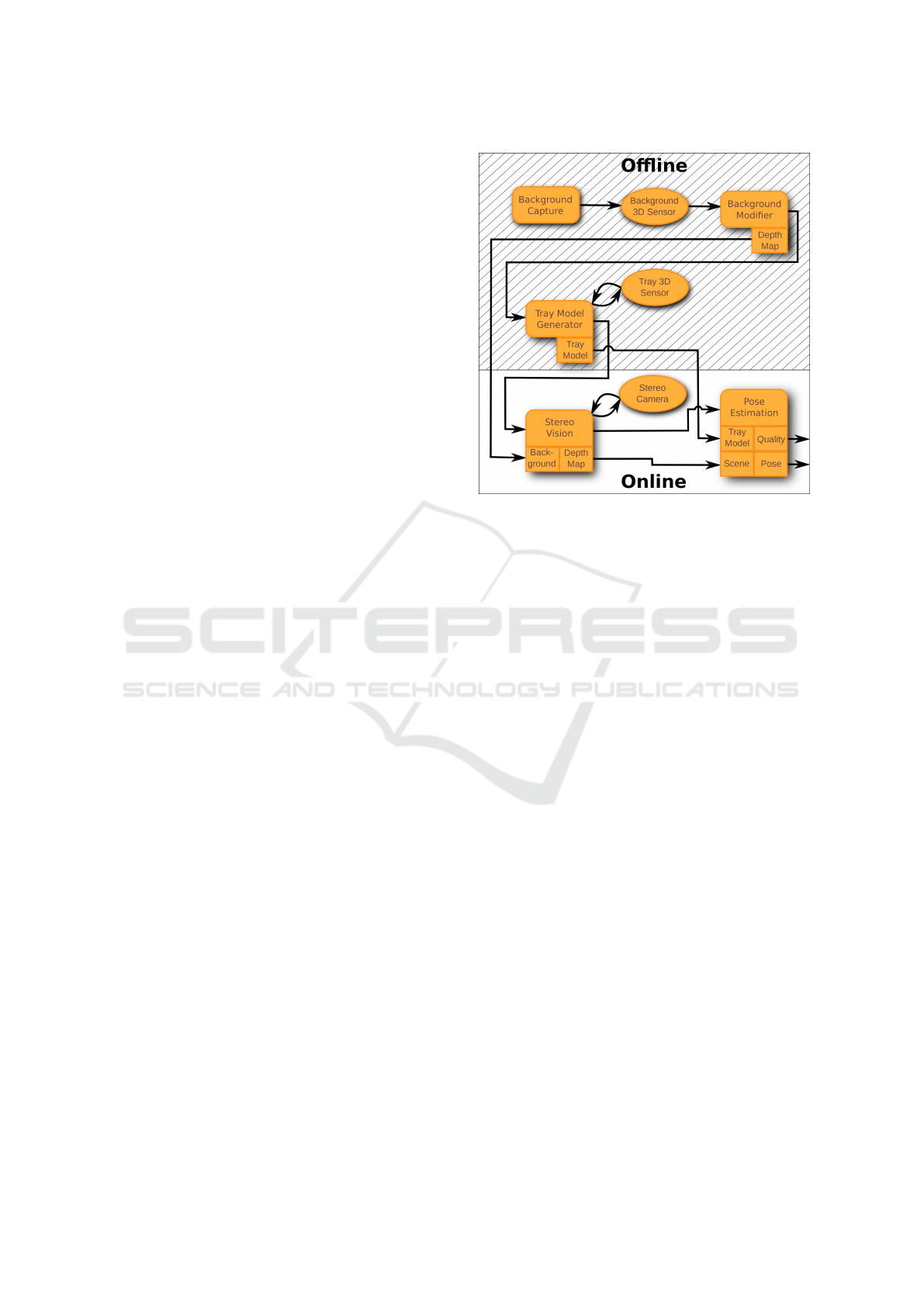
Figure 2: Overview of the pose estimation pipeline. Round

elements indicate sensors, square elements indicate soft-

ware blocks and the sub-boxes indicate signals and data

transfer between the software blocks.

3 THE SIMULATION SYSTEM

In this section, we introduce the elements of the pose

estimation pipeline shown in Figure 2. The pipeline

can be seen as a function evaluation, f (x), where

the ﬁnal “Quality” corresponds to the value of the

function.

The vector x = (r, α, BL, β)

corresponds to the 4

variables shown in Figure 1, r is the radial distance, α

is the polar angle, BL is the baseline and β is the ver-

gence. Furthermore, the sensor always points towards

the center of the table with the tray. In order to ﬁnd

good camera placements, basic optimization methods

can then be used to adjust x, to ﬁnd the highest quality

f (x).

Now that the overall approach is described, we

will go into more detail with the individual parts of the

pose estimation pipeline. The ﬁrst step is to generate

a background depth map, which can be used for back-

ground removal. To achieve this, the “Background

Capture” block removes the tray from the scene and

requests the “Background 3D sensor” to capture a

depth map of the scene. This depth map is given to

the ”Background Modiﬁer” block, which dilates the

background to help reduce the effect of noise. After-

wards, the modiﬁed depth map is made available for

the “Stereo Vision” block, and the “Tray Model Ge-

nerator” block is activated.

To model the object, a point cloud has to be cap-

Simulation-based Optimization of Camera Placement in the Context of Industrial Pose Estimation

527

tured from several viewpoints. Furthermore, the tray

contains several slots, for placing items. Examples

where the slots are empty and full also have to be con-

sidered in the overall object model. The object model

is generated by removing all of the scene except the

tray, and all the items in the tray. Then point clouds

are captured from all viewpoints using the “Tray 3D

Sensor”. In this work, we use 6 viewpoints, where the

object is rotated around the z-axis in steps of 60

◦

, this

was chosen to cover the object without producing too

much overlap. For each viewpoint (slots + 1) point

clouds are captured to model the effects of whether

the slots are empty or not. This is done by ﬁrst cap-

turing a point cloud of the tray containing all items.

Then the closest item is iteratively removed until the

tray is empty. In our case the trays we test have

4 and 8 slots. After all the point clouds are captu-

red, they are down-sampled to the surface resolution,

SRes, (see Table 1).

The next step in the “Tray Model Generator”

block is to compute point features. In this work, the

ECSAD feature (Jørgensen et al., 2015) is used. The

features are computed on each of the individual point

clouds in the model. After the features are compu-

ted, the point clouds are combined into a single point

cloud and feature cloud pair, which can be used in the

RANSAC algorithm.

Besides just building a point cloud model for the

initial pose estimation, we also build a set of point

clouds for ﬁne tuning the pose with ICP. This is done

by generating a point cloud for each view point, by

simply combining the point clouds with differently

ﬁlled slots into one. Then the combined point cloud

is down-sampled to the surface resolution. Lastly, the

view points of the ICP point clouds are stored, such

that they can be used to determine which of the 6 point

clouds should be used for the ICP algorithm. An ex-

ample of an ICP point cloud can be seen in Figure 4,

where it is used to indicate the believed pose of the

tray.

When the model is generated it is made available

for the “Pose Estimation” block, and the “Stereo Vi-

sion” block is activated. This block generates a point

cloud based on a set of captured stereo images, accor-

ding to Section 4. After a point cloud is generated, it

is made available for the “Pose Estimation” block.

Finally, the “Pose Estimation” block determines

the pose of the object according to Section 5. During

this computation, four quality metrics are computed,

namely the positional error, the rotational error, the

number of correct feature matches and whether the

pose estimation was a success or not. A success is de-

ﬁned as a pose estimate, where the positional error is

less than 3mm and the rotational error is less than 5

◦

These values are chosen to ensure a fairly precise pose

is known for future manipulation tasks. A correct fea-

ture match is deﬁned to be a match where the features

based on the ground truth transformation are less than

4.5mm apart from each other. This distance is chosen

slightly bigger than the success requirement, since the

feature matches are an indicator of the pose estima-

tion quality, and here it turned out a slightly larger

radius produced a higher correlation between feature

matches and success rate.

To wrap the entire pipeline into a function with

some statistical signiﬁcance, we evaluate it for multi-

ple scenarios. The differences between the scenarios

are the placement of the tray, the ﬁlling of the tray

and the placement of the lighting. For each evaluation

we evaluate the off-line part, in Figure 2, 250 times.

Each of the 250 evaluations returns the four men-

tioned quality metrics, which are analyzed to com-

pute the success rate, the average feature matches, the

average positional error and the average rotational er-

ror.

4 SENSORS - SIMULATION AND

REAL WORLD

In this work, we test two different stereo vision met-

hods for generating the point clouds used during pose

estimation. The ﬁrst method is to project a rando-

mized pattern on the scene, to get more texture, and

then use the “LibElas” (Geiger et al., 2010) stereo vi-

sion algorithm to generate a depth map. We refer to

this method as the one shot method. Examples of a

real and simulated image and the corresponding depth

maps for this method are shown in Figure 3.

The second method is a 12 shot structured light

approach, here a phase shift pattern consisting of 12

different sinusoidal images are projected on the scene.

The point cloud is then generated based on the 12 re-

sulting stereo image pairs and phase-unwrapping of

the projected pattern (Huntley and Saldner, 1993).

Both sensors are simulated in VEROSIM using

cameras with a resolution of 640x480 and a horizontal

ﬁeld of view of 43

◦

. The projected light is simulated

by an OpenGL-based projector with a changeable pat-

tern (Everitt, 2001). After the images are captured,

noise and smoothing are added to make the images

more realistic. In particular, we add uniform random

noise with a range of ±10 to each pixel, and then we

smooth the image with a mean ﬁlter over 3x3 pixels.

As seen in Section 6, the one shot stereo approach

gave the most robust results in simulation. Therefore,

we chose this method for the real world validation. In

VISAPP 2018 - International Conference on Computer Vision Theory and Applications

528

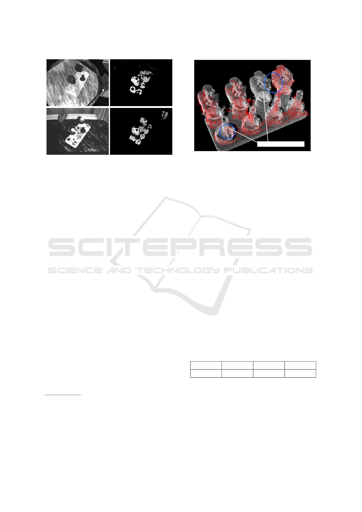
a b

c d

Figure 3: Simulated and real images. a) shows the simu-

lated left camera image. b) shows the corresponding depth

map after background subtraction. c) shows the real left

camera image. d) shows the corresponding depth map.

the real world tests we used a “Bumblebee” camera

and a “Qumi” projector

. As seen in Figure 3 there

are some differences between the 2D images, but the

resulting depth maps are similar.

5 POSE ESTIMATION

In Section 3, we discussed how the tray model was

generated, such that it is ready to use for a RANSAC

algorithm. In Section 4 we discussed how the point

clouds of the scene are generated. Now to apply the

pose estimation, the ﬁrst step is to down-sample the

scene cloud to surface resolution, SRes, and compute

the ECSAD features for the scene. After the featu-

res are computed, they are matched to the tray model

using a k nearest neighbor search (k is given in Ta-

ble 1).

The next step is to reject inconsistent feature ma-

tches, this is done by ensuring that the z-coordinate

of the object feature corresponds to scene features

placed similarly above the table within a band of

±20mm. Now that the feature matches are prepared

we use a slightly modiﬁed version of a RANSAC al-

gorithm presented by Buch et al. (Buch et al., 2013).

The modiﬁcation we add is a quick rejection step,

which occurs if the guessed pose does not correspond

to the tray being placed on the table. This is determi-

The camera used is a “Bumblebee” with a 43

◦

HFOV

and a resolution of 1024x768 - https://eu.ptgrey.com/

bumblebee2-08-mp-mono-ﬁrewire-1394a-6mm-sony-

icx204-2-eu

The projector is a “Qumi Q5-WT” with a re-

solution of 1280x800 - http://www.vivitek.eu/Category/

Pocket-Personal-Projectors/3/Qumi-Q5

Objects missing in the scene

Figure 4: Pose estimation of the tray, the red points are the

scene cloud and the white points are an up-sampled ver-

sion of the tray cloud used during ICP. Notice the encircled

areas, where it can be seen that the partially see-through

model helps to produce more inliers when items are mis-

sing.

ned based on a threshold that allows the object to be

placed ±20mm above the table, and with an error on

rotation of less than ±10

◦

In the RANSAC algorithm, we evaluate the ﬁtness

of the guesses based on an inlier count, which is de-

termined based on the scene and an ICP model. The

ICP model is chosen as the one, which view point is

closest to the scene view point. The number of RAN-

SAC iterations, RIt, is given in Table 1.

After a match is found, the ﬁnal step is to run an

ICP algorithm to ﬁne tune the pose. This is done by

selecting the ICP model, which view point is closest

to the scene view point. The ICP algorithm runs for

ICPIt iterations or until convergence. An example of

a pose estimate after ICP is given in Figure 4.

All the key parameters of the pose estimation al-

gorithm is given in Table 1. SRes are chosen based on

(Jørgensen et al., 2015). k, RIt and ICPIt are chosen

to be fairly high compared to (Jørgensen et al., 2015).

This ensures a higher success rate at the cost of com-

putation time.

Table 1: Pose estimation parameters.

SRes k RIt ICPIt

2.0mm 25 100000 100

6 RESULTS - OPTIMIZATION IN

SIMULATION

Several steps were taken, to determine good solutions

based on optimization. The ﬁrst was to plot the ob-

jective function surfaces. This was done by varying

Simulation-based Optimization of Camera Placement in the Context of Industrial Pose Estimation

529

◦

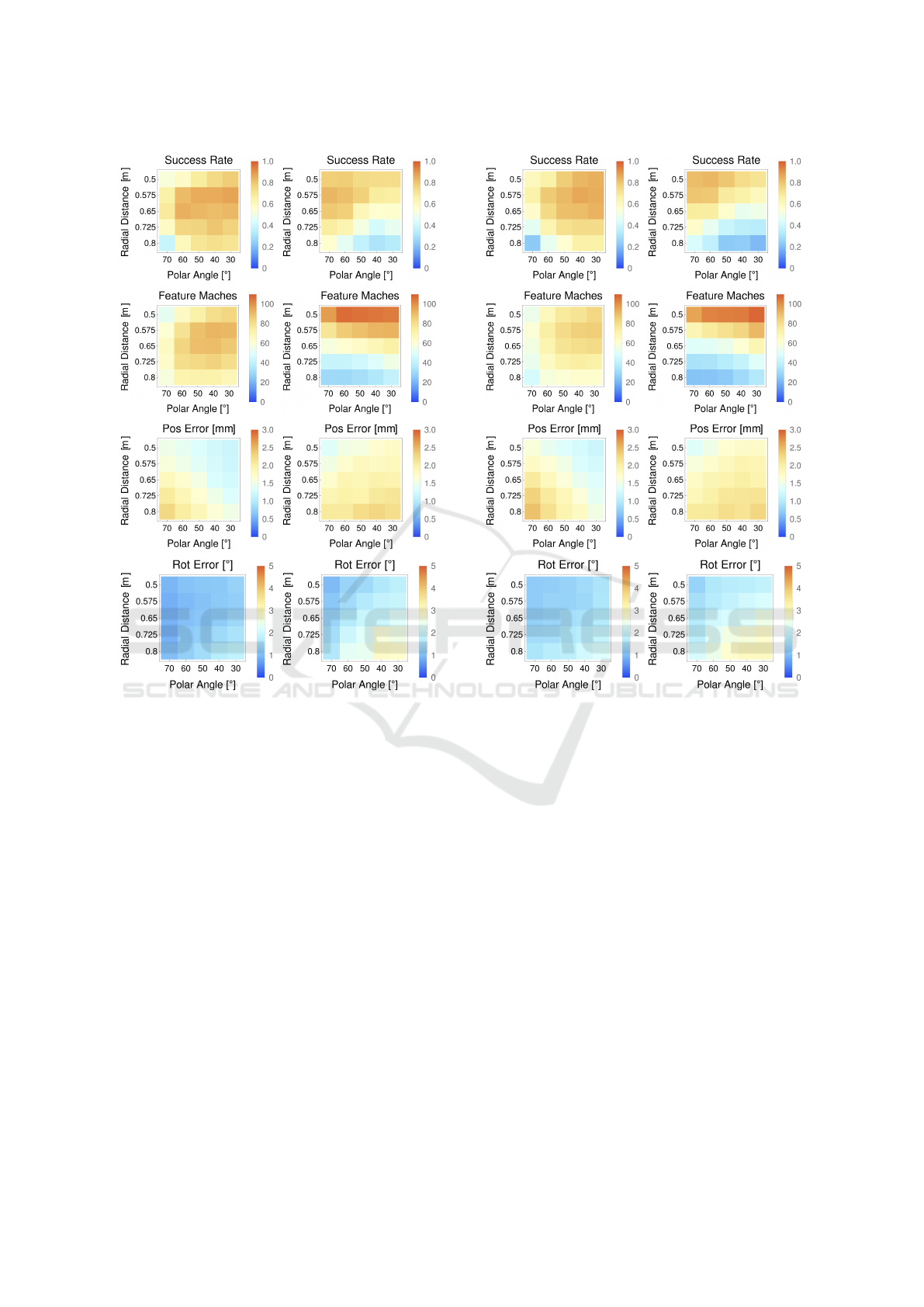
Figure 5: Brute force optimization for the 8 slot tray. The

left side shows the result for one shot stereo, and the right

side shows the results for 12 shot structured light. The green

circles indicate where the success rate is highest.

the radial distance and the polar angle of the camera

system (see Figure 1) and then plotting the resulting

quality measures. The plots for the tray with 8 slots

are shown in Figure 5 and the plots for the tray with

4 slots are shown in Figure 6. Both dimensions were

sampled in 5 steps and for each point, 250 simulati-

ons were evaluated to enable statistical analysis of the

results. This corresponds to 5x5x250 = 6250 simula-

tions to generate values for the surface.

The results show that the one shot approach tends

to produce the best pose estimation results in terms

of success rate (see Figure 5 and 6, a and b). But

the 12 shot approach tends to produce more precise

point clouds when the camera is close to the object.

Unfortunately, they also contain more outliers. This is

seen by the higher number of correct feature matches

for the 12 shot approach when the camera is close. It

should be noted that the two different trays produce

quite similar plots, so the same camera position can

◦

Figure 6: Brute force optimization for the 4 slot tray. The

left side shows the result for one shot stereo, and the right

side shows the results for 12 shot structured light. The green

circles indicate where the success rate is highest.

be used for both trays. But the camera placement is

quite sensitive to the method that is used to generate

the point clouds, thus the system should be optimized

dependent on the method.

The results also show the number of correct fea-

ture matches (see Figure 5 and 6, c and d). The pur-

pose of this score was to test if it could be used to pre-

dict the success rate of a given camera position. This

would be beneﬁcial, since it requires less computation

to determine. Furthermore, it is not a binary value so

it is less affected by quantiﬁcation compared to the

success/fail value. For the one shot approach there is

a weak correlation, but for the 12 shot approach there

is no correlation. Thus we decided not to pursue this

further, but in the one shot approach it could be used

to narrow the search area.

The plots also show the positional error and the ro-

tational error (see Figure 5 and 6, e, f, g and h). Here it

becomes clear that the positional error is a bottleneck,

VISAPP 2018 - International Conference on Computer Vision Theory and Applications

530

and the plots of positional error and success rate are

anti-correlated for both image sensors.

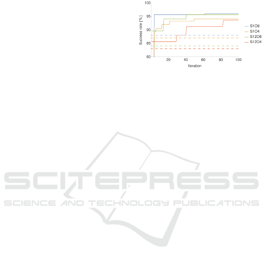
Besides simply doing brute force optimization of

the 2 parameters, we also used the optimization met-

hod “RBFopt” (Costa and Nannicini, 2015) to deter-

mine sensor placements that maximize the success

rate. This search method enabled us to optimize the

radial distance, the polar angle, the base line and the

vergence. In Figure 7, the success rate as a function

of the optimization iterations is shown. Here it can

be seen that a success rate of 96% is achieved when

4 parameters are optimized. This is higher than the

success rate of the brute force search on two parame-

ters, which only reached 88%, thus it is beneﬁcial to

optimize more than the two parameters in the brute

force search. This is one of the reasons simulation-

based optimization is a powerful tool, since this type

of search would be unfeasible in the real world. One

way to do the search in the real world is to place 250

objects on a table and capture them from the ﬁrst view

point, then the success rate would have to be determi-

ned based on manual interaction. This would have to

be done for all 100 iterations of the sequential opti-

mization algorithm, which would be very time con-

suming. An alternative would be to make an auto-

mated system that could move the sensors and then

simply capture the same dataset from all sensor posi-

tions. Unfortunately, this process requires a parallel

approach to optimization. If a brute force method is

chosen this would require 625 positions for a quanti-

ﬁcation of 5 steps per parameter, which again would

make it quite time consuming.

The optimization based on RBFopt again shows

that the one shot approach produces the most robust

solution. For the tray with 8 slots using the one shot

method, the optimal parameters are a radial distance

of 605mm, a polar angle of 32

◦

, a vergence of 3.5

◦

and a baseline of 81mm. The main reason for the im-

provement is the reduced baseline, which originally

was 120mm. The reduced baseline makes the mat-

ching task easier and increases the overlap of the ima-

ges, which makes the region covered by the resulting

depth map larger.

7 RESULTS - REAL WORLD

TRIALS

After the problem was optimized in simulation, we

tested the relevance of the simulation based on real

world trials. This was done by generating 2D plots

for the quality measures, as a function of the radial

distance and the polar angle. These plots are similar

to the simulated case using the one shot method and

Figure 7: Optimization of the success rate by tuning the 4

camera parameters using RBFopt. S1 refers to using the one

shot method and S12 refers to using the 12 shot method. O8

refers to that 8 items can be placed in the tray and O4 refers

to that 4 items can be placed in the tray. The dashed lines

correspond to the success rate of the optimal placements

from the brute force search over 2 parameters.

the 8 slot tray, the plots are shown for comparison in

Figure 8.

The real world plots were generated based on the

robotic setup shown in Figure 1. The robot was con-

ﬁgured to 25 positions, such that the sensor posi-

tion roughly matched the position used in simulation.

Then the tray was placed on the table 100 times, such

that the item conﬁguration matched that of the simu-

lated images. For each placement the robot was mo-

ved between the 25 positions, and for each position

an image pair was taken.

Then point clouds were generated based on the

stereo images. These were then mapped to the simu-

lation scene, such that the table plane could be used

as a constraint during pose estimation. Afterwards, a

rough estimate of the cameras transformations was at-

tached to the scene for each view point, and a ground

truth label was attached to the ﬁrst view point for all

100 object placements. Next, the ground truth poses

were mapped to the other 24 view points, and ICP

was used to ﬁne tune the object poses. Then the ca-

mera poses were ﬁne tuned to minimize the error be-

tween the individual object poses and the average ob-

ject pose over the 25 view points. This was done ite-

ratively until the error between individual object po-

ses and the average object pose had reached a sub-

millimeter level. The average pose of the objects was

then used as the ground truth pose, to avoid biasing

the ground truth based on the same ICP that is used

in the pose estimation algorithm. Now, a dataset with

high precision ground truth labels was available, and

lastly the pose estimation algorithm was used on the

dataset to determine the quality measures in Figure 8.

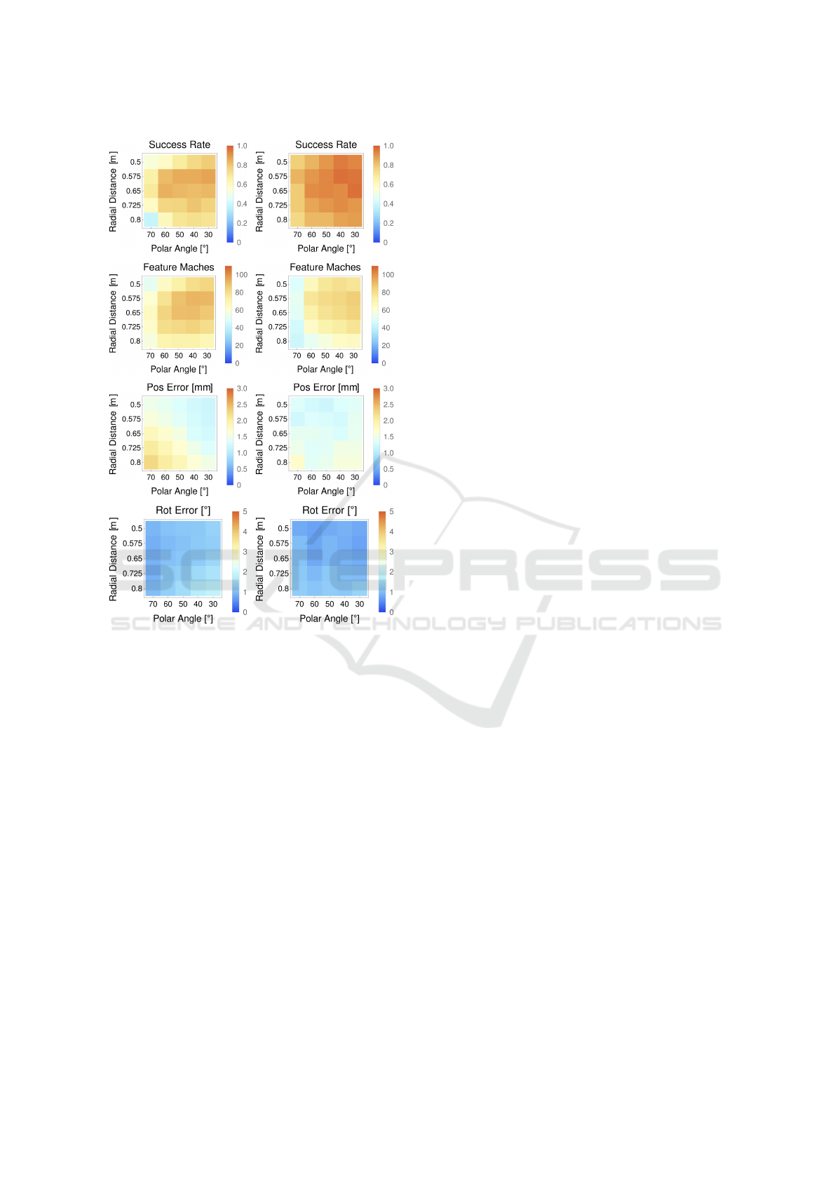
In Figure 8 it can be seen that there are some de-

viations between the simulated results and the real

world results. In general, the performance of the pose

Simulation-based Optimization of Camera Placement in the Context of Industrial Pose Estimation

531

◦

Figure 8: Brute force optimization for the 8 slot tray. The

left side shows the result for one shot stereo in simulation

and the right side shows the real world equivalent. The

green circles indicate where the success rate is highest.

estimation is slightly better in the real world, this is

likely because more variation was added in the si-

mulation, to ensure the solutions are robust. Thus,

the quality of the point clouds from simulation varied

more and contained more low quality point clouds,

which made the overall success rate in simulation go

down. The main difference is the background illumi-

nation, which was nearly constant in the real world

experiments, but varied signiﬁcantly in the simulated

experiments.

Another deviation is that the positional and rota-

tional errors are weakly correlated to the results in

simulation (see Figure 8, e, f, g and h). But since

the errors in the real world are quite small, it indicates

that the main source of failures is caused by RANSAC

supplying a poor estimate for ICP. Thus, highly accu-

rate simulation-based predictions of positional and ro-

tational errors are less important when determining

camera positions with a high success rate.

Overall the best positions in the simulated expe-

riments are also good in the real world, which is the

most important aspect when using simulation for opti-

mization. Thus, it is an indication that the overall ap-

proach is valid, for determining camera placements.

8 CONCLUSION AND FUTURE

WORK

In this work, a simulation system for industrial

pose estimation problems was built, to maximize the

success rate by adjusting the camera placement. The

results show that the success rate signiﬁcantly de-

pends on the camera placement, especially for a dif-

ﬁcult task where the tray is very bright and the items

in the tray are very dark. Furthermore, geometric pro-

perties of the object also inﬂuence the quality of the

pose estimation.

Overall we were able to ﬁnd decent solutions in

simulation. For a “Bumblebee” camera, we achieved

a success rate of 88%, based on brute force optimiza-

tion. By using sequential optimization, we show that

a success rate of 96% can be achieved if the base line

of the camera is also adjusted.

Lastly, we tested the pose estimation pipeline in

the real world. Here the optimal camera placement

roughly matched the optimal camera placement in si-

mulation. At the optimal placement in simulation a

success rate of 96% is achieved in the real world. At

the best placement in the real world a success rate of

97% was achieved.

In the work, we showed that the simulation tool

was helpful in designing the case speciﬁc pose estima-

tion algorithm, both as a tool to determine important

poses as well as to quickly evaluate what was required

to make the partially see through view based tray mo-

del complete enough to achieve good pose estimation

results.

In summary, we have shown that we can transfer

the problem of ﬁnding suitable camera placements for

industrial pose estimation to simulation. By that, we

can provide a tool that can signiﬁcantly reduce the

set-up times of robot solutions and by that can faci-

litate the application of vision based robot solutions

in industry, a problem recognized to be crucial for in

particular SMEs (Kr

uger et al., 2014).

ACKNOWLEDGMENT

The ﬁnancial support from the The Danish Innovation

Foundation through the strategic platform MADE-

VISAPP 2018 - International Conference on Computer Vision Theory and Applications

532

Platform for Future Production and from the EU

project ReconCell (FP7-ICT-680431) is gratefully

acknowledged.

REFERENCES

Aldoma, A., Marton, Z.-C., Tombari, F., Wohlkinger, W.,

Potthast, C., Zeisl, B., Rusu, R. B., Gedikli, S., and

Vincze, M. (2012). Tutorial: Point cloud library:

Three-dimensional object recognition and 6 dof pose

estimation. IEEE Robotics & Automation Magazine,

19(3):80–91.

Buch, A. G., Kraft, D., Kamarainen, J.-K., Petersen, H. G.,

and Kr

uger, N. (2013). Pose estimation using local

structure-speciﬁc shape and appearance context. In

Robotics and Automation (ICRA), 2013 IEEE Inter-

national Conference on, pages 2080–2087. IEEE.

Chen, S., Li, Y., and Kwok, N. M. (2011). Active vi-

sion in robotic systems: A survey of recent develop-

ments. The International Journal of Robotics Rese-

arch, 30(11):1343–1377.

Costa, A. and Nannicini, G. (2015). Rbfopt: an open-

source library for black-box optimization with costly

function evaluations. Under review.

Dong, Y., Hutchens, T., Mullany, B., Morse, E., and Da-

vies, A. (2014). Using a three-dimensional opti-

cal simulation to investigate uncertainty in image-

based dimensional measurements. Optical Engineer-

ing, 53(9):092007–092007.

Everitt, C. (2001). Projective texture mapping. White paper,

NVidia Corporation, 4.

Geiger, A., Roser, M., and Urtasun, R. (2010). Efﬁcient

large-scale stereo matching. In Asian conference on

computer vision, pages 25–38. Springer.

Großmann, B., Siam, M., and Kr

uger, V. (2015). Compa-

rative Evaluation of 3D Pose Estimation of Industrial

Objects in RGB Pointclouds, pages 329–342. Springer

International Publishing, Cham.

Huntley, J. M. and Saldner, H. (1993). Temporal phase-

unwrapping algorithm for automated interferogram

analysis. Applied Optics, 32(17):3047–3052.

Irgenfried, S., Tchouchenkov, I., W

orn, H., Koci, R., Hana-

cek, P., Kunovski, J., Zboril, F., Samek, J., and Pe-

ringer, P. (2011). Cadavision: a simulation frame-

work for machine vision prototyping. In Proceedings

of the Second International Conference on Computer

Modelling and Simulation, pages 59–67.

Jørgensen, T. B., Buch, A. G., and Kraft, D. (2015). Ge-

ometric edge description and classiﬁcation in point

cloud data with application to 3d object recognition.

In Proceedings of the 10th International Conference

on Computer Vision Theory and Applications (VISI-

GRAPP), pages 333–340.

Knoop, S., Vacek, S., and Dillmann, R. (2006). Sensor fu-

sion for 3d human body tracking with an articulated 3d

body model. In Robotics and Automation, 2006. ICRA

2006. Proceedings 2006 IEEE International Confe-

rence on, pages 1686–1691. IEEE.

Kouteck

y, T., Palou

sek, D., and Brandejs, J. (2015). Ap-

plication of a reﬂectance model to the sensor planning

system. In SPIE Optical Metrology, pages 953005–

953005. International Society for Optics and Photo-

nics.

uger, N., Ude, A., Petersen, H. G., Nemec, B., Ellekilde,

L.-P., Savarimuthu, T. R., Rytz, J. A., Fischer, K.,

Buch, A. G., Kraft, D., et al. (2014). Technologies

for the fast set-up of automated assembly processes.

KI-K

unstliche Intelligenz, 28(4):305–313.

Mavrinac, A., Chen, X., and Alarcon-Herrera, J. L. (2015).

Semiautomatic model-based view planning for active

triangulation 3-d inspection systems. IEEE/ASME

Transactions on Mechatronics, 20(2):799–811.

Medeiros, E., Doraiswamy, H., Berger, M., and Silva, C. T.

(2014). Using physically based rendering to bench-

mark structured light scanners. In Computer Graphics

Forum, volume 33, pages 71–80. Wiley Online Li-

brary.

Nilsson, J., Ericsson, M., and Danielsson, F. (2009). Virtual

machine vision in computer aided robotics. In 2009

IEEE Conference on Emerging Technologies & Fac-

tory Automation, pages 1–8. IEEE.

Papazov, C. and Burschka, D. (2010). An efﬁcient ransac

for 3d object recognition in noisy and occluded sce-

nes. In Asian Conference on Computer Vision, pages

135–148. Springer.

Rios, L. M. and Sahinidis, N. V. (2013). Derivative-free op-

timization: a review of algorithms and comparison of

software implementations. Journal of Global Optimi-

zation, 56(3):1247–1293.

Rossmann, J., Steil, T., and Springer, M. (2012). Valida-

ting the camera and light simulation of a virtual space

robotics testbed by means of physical mockup data.

In International symposium on artiﬁcial intelligence,

robotics and automation in space (i-SAIRAS), pages

1–6.

Rozantsev, A., Lepetit, V., and Fua, P. (2015). On rendering

synthetic images for training an object detector. Com-

puter Vision and Image Understanding, 137:24–37.

Schluse, M., Schlette, C., Waspe, R., and Roßmann, J.

(2013). Advanced 3d simulation technology for ero-

botics: Techniques, trends, and chances. In 2013 Sixth

International Conference on Developments in eSys-

tems Engineering, pages 151–156.

Takei, S., Akizuki, S., and Hashimoto, M. (2014). 3d object

recognition using effective features selected by evalu-

ating performance of discrimination. In Control Au-

tomation Robotics & Vision (ICARCV), 2014 13th In-

ternational Conference on, pages 70–75. IEEE.

Ye, M., Wang, X., Yang, R., Ren, L., and Pollefeys, M.

(2011). Accurate 3d pose estimation from a single

depth image. In Computer Vision (ICCV), 2011 IEEE

International Conference on, pages 731–738. IEEE.

Simulation-based Optimization of Camera Placement in the Context of Industrial Pose Estimation

533