Robust Plant Segmentation from Challenging Background with a

Multiband Acquisition and a Supervised Machine Learning

Algorithm

Taha Jerbi, Aaron Velez Ramirez and Dominique Van Der Straeten

Laboratory of Functional Plant Biology, Dept. of Biology, Ghent University, K. L. Ledeganckstraat 35, 9000 Gent, Belgium

Keywords: Image Processing, Plant Phenotyping, Classification, Segmentation, Multispectral Acquisition, Supervised

Learning, Arabidopsis.

Abstract: Remote sensing through imaging forms the basis for non-invasive plant phenotyping and has numerous

applications in fundamental plant science as well as in agriculture. Plant segmentation is a challenging task

especially when the image background reveals difficulties such as the presence of algae and moss or, more

generally when the background contains a large colour variability. In this work, we present a method based

on the use of multiband images to construct a machine learning model that separates between the plant and

its background containing soil and algae/moss. Our experiment shows that we succeed to separate plant parts

from the image background, as desired. The method presents improvements as compared to previous methods

proposed in the literature especially with data containing a complex background.

1 INTRODUCTION

Accurate segmentation of plants from the image

background is the first step for the extraction of traits

in phenotyping applications and precision agriculture.

An intuitive approach that simplifies the task by

covering the soil (Arend et al., 2016) could be the

easiest solution making the segmentation

straightforward; however, this solution is not

practical in field applications. Moreover, it could

perturb the gas exchange between the soil and the air

in laboratory experiments. Image processing based on

algorithms which succeed to overcome application-

specific difficulties offers solutions to extract plant

traits. Image segmentation difficulties include: (a)

large variability of the soil colour, (b) the presence of

moss and algae with colours similar to the plant to

segment, (c) the presence of non-green plant parts as

flowers and/or yellow and brown parts of leaves of

senescing plants or in stressed plants, which can

occur in phenotyping experiments under specific

conditions.

Previous work tackled this problem mainly by

considering a classification problem on the colour

space. Sharr (Sharr et al., 2016) presents four

segmentation methods from different universities and

research laboratories (Leibniz Institute of Plant

Genetics and Crop Plant Research-IPK-Germany,

Nottingham University-United Kingdom, Michigan

State University-United States, and Wageningen

University-Netherlands) in a challenge frame. The

first method uses a 3D histogram cube to encode the

probability for each observed pixel in the training

data of belonging to the plant or background. The

second method is based on a superpixel segmentation

in Lab colour space as a first step, and thresholding of

the superpixel image in the second step. In the third

method, the foreground/background segmentation is

done by a simple empirical threshold on the ‘a’

channel of the Lab colour space. The fourth method

uses an artificial neural network (ANN) with one

hidden layer for plant/background separation. In

general, for all these methods and as mentioned in the

paper (Sharr et al., 2016), the results show that “most

methods perform well in separating plant from

background, except when the background presents

challenges” (Sharr et al., 2016). A similar approach

using the watershed algorithm was also proposed in

an earlier study for plant segmentation from

background (Åstrand et al., 2006).

In (De Vylder et al., 2012), the authors used the

Expectation Maximization (EM) algorithm with the

hue signal of the images to characterize two

Gaussians distributions modeling the plant and the

Jerbi T., Velez Ramirez A. and Van Der Straeten D.

Robust Plant Segmentation from Challenging Background with a Multiband Acquisition and a Supervised Machine Learning Algorithm.

DOI: 10.5220/0006552001000105

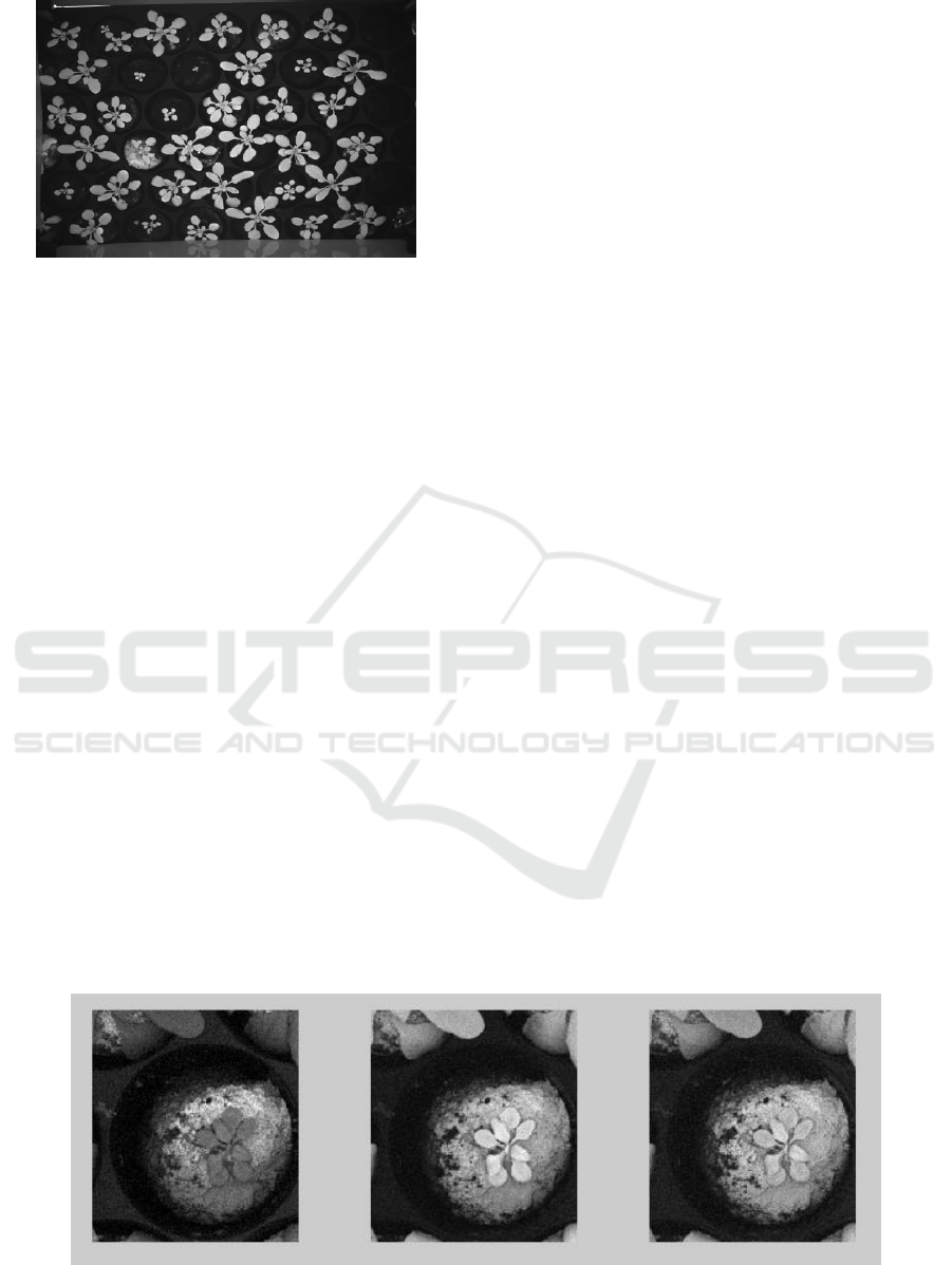
Figure 1: System acquisition of Arabidopsis plants.

background in the histogram. However, this method

will also face difficulties when the hue signal of the

plant and the background are similar.

More recently, machine learning approaches have

been used to segment plants from soil (Navarro et al.,

2016), but the images used were the Red-Green-Blue

(RGB) and the Near Infra-Red (NIR) and the

segmentation was done separately for the RGB and

NIR. In this study, a comparison between three

machine learning approaches (k-nearest neighbor

(kNN), naive Bayes classifier (NBC), Support Vector

Machine (SVM)) showed that SVM performed better

for the NIR, while kNN segmentation was better for

the colour images (RGB).

The majority of algorithms cited above use either

one channel or the three colour channels RGB except

the fourth algorithm cited in (Sharr et al., 2016) that

uses also an excessive green value (R,2G,B) with two

texture features, and the machine learning approach

in (Navarro et al., 2016) that uses the NIR signal.

However, in phenotyping applications, more signals

are generally acquired to observe the plant response

to different wavelengths including fluorescence

signals. In addition to their biological meaning, these

data can also be useful for the plant segmentation. In

our project, which is part of the TIMESCALE

project-Horizon 2020, 14 bands are used to observe

the plants’ responses to different environmental

conditions. These bands are used in our segmentation

approach as discussed below. In the next section, we

present our acquisitions and the algorithm proposed

for a better segmentation of the plant from a

challenging background. In section 3, we evaluate our

results and discuss the different methods.

2 MATERIALS AND METHODS

2.1 Materials and Data

Our phenotyping platform is composed by a table, a

robot, an acquisition system (lighting system, filters

and cameras) and software that automatically

acquires images during a biological experiment. The

acquisition system is composed by cameras and filters

that allow acquisition at specific wavelengths.

Chlorophyll fluorescence signals allow to study plant

photosynthesis (Baker, 2008). The system flashes a

specific wavelength in a very short interval of time

and captures the emitted signal by the plant

photosynthetic apparatus. Our system allows to

measure these signals in different phases: an excited

phase when the plant is under light and a non-excited

phase when the plant is in darkness. Different bands

are either directly acquired by the camera and the

filter system or computed from the acquired bands.

These signals and their biological interpretations are

described in (Baker, 2008) and in (Gitelson et al.,

1999). For each acquisition, the robot moves the

acquisitions system (cameras and filters) on top of a

plate containing plants and acquires images. All

bands can be acquired in less than 2 minutes, and we

assume there is no modification of the scene during

this short period of time (no shape or position

variation).

Figure 2: Acquisition of an Arabidopsis plant with 3 different bands of the system, the differentiation between the plant and

the algae/moss is difficult with each wavelength band shown.

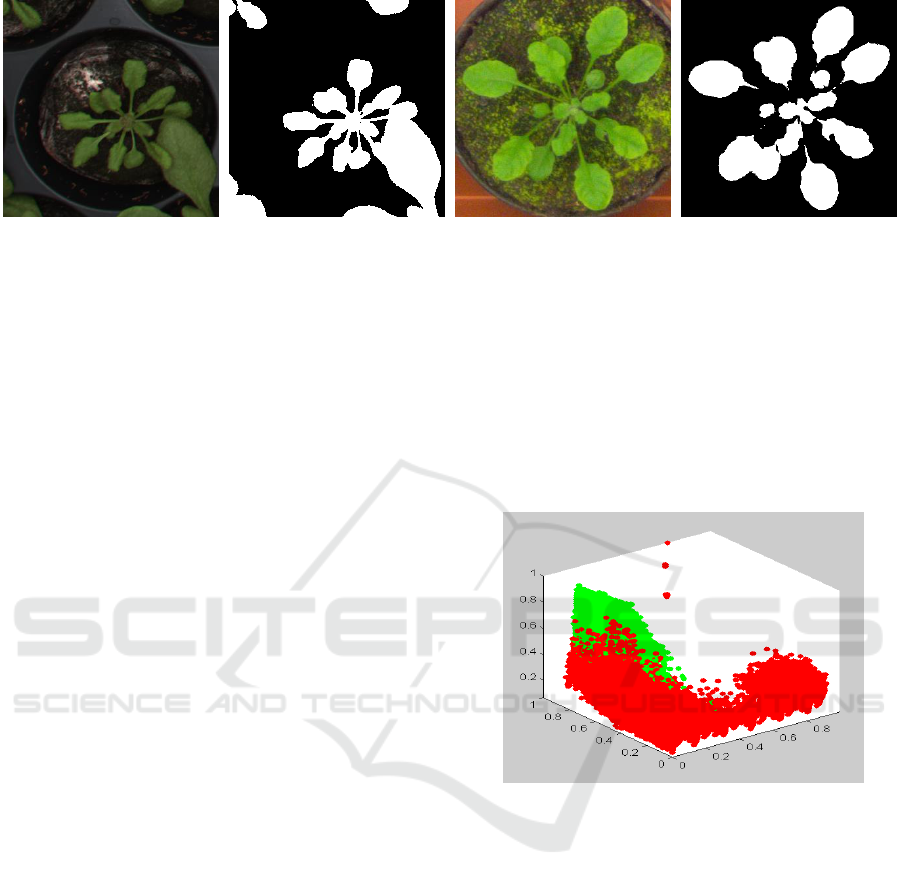
(a) (b) (c) (d)

Figure 3: Plant segmentation in presence of moss and algae: (a) Plant from our database, (b) Our automatic segmentation

(RF), (c) Plant from the database of (Scharr, 2016), (d) Our automatic segmentation (SVM Gaussian).

In our experiment, plants were imaged from day 5

after sowing (Das 5) to Das 22. For the purpose of the

biological experiment, some plants were under

drought stress. The system generated approximate-

vely 30000 acquisitions (14 images each) for an

experiment that takes 22 days. Each image contains

36 plants.

2.2 Method

First, as a pre-processing step, the images were split

into smaller images containing one plant each. We

considered 115 images to form our database. If

needed, images were downsized to have pixel to pixel

correspondence between all bands. In addition to the

14 bands registered, 6 more bands were computed:

the HSV (3 bands that represent the colour images as

Hue, Saturation and Value), and to include informa-

tion about the neighbors of a pixel, we also computed

the median value in a 15 pixels large square (H15,

S15 and V15) using a median filter. Altogether, 20

features are available to characterize the plants and

the background (soil, moss and algae) pixels in the

image.

In our approach, pixel classification is used as a

method for plant segmentation. To overcome the

difficulties of the plant separation from a complex

background, supervised machine learning approaches

bring a solution to have a specific model to a

particular dataset. In fact, if the dataset contains

plants with flowers, the model constructed will be

different from a model constructed from plants with

just leaves for example. Two main supervised

machine learning approaches were used in this work,

the support vector machine algorithm (SVM) and the

random forest algorithm (RF).

SVM is a supervised machine learning approach

that was introduced by Vapnik and Cortes (Cortes and

Vapnik, 1995). The method is based on two steps. In

the first one (learning or training step), based on pre

labelled samples, the algorithm constructs borders to

separate data into classes (regions) defined by the

predefined labels (figure 4.). It also ensures maximum

margins between the borders and the samples in order

to reduce errors when applying these borders to new

data. In the second step (prediction step), the model

(borders) is applied to the new data to predict the

classes of the new input.

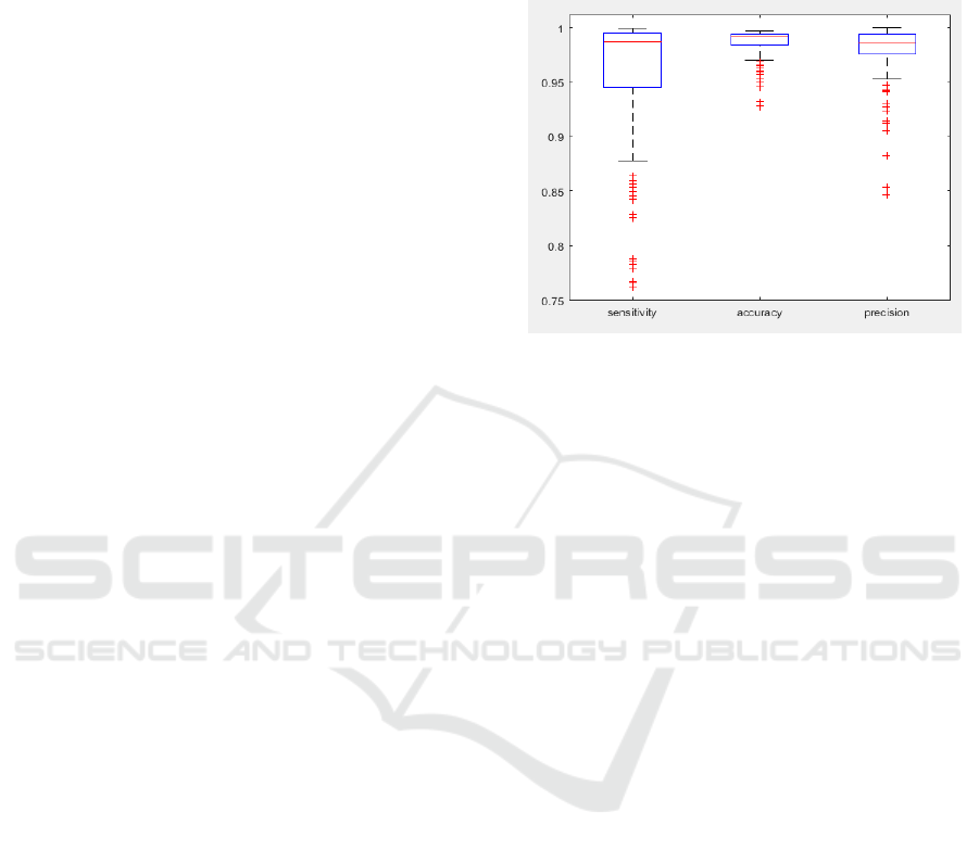
Figure 4: Training data representation in 3D: plant data in

green and background data in red (only RGB colour

features are represented). Dataset: Ara2013 (Scharr et al.,

2016), Number of images: 10/165.

Random Forest (RF) algorithm (Breiman, 2001)

is also a supervised algorithm. It is based on the idea

of using the decision trees where each tree is

constructed using bootstrapped random variables. In

each tree node, the decision is taken according to the

best among random predictors. By generating

multiple trees, the random forest algorithm is

obtained. At the end of the algorithm, the forest (all

the trees) takes a decision corresponding to the global

vote of its trees.

In order to construct our models with both

methods, the pixel values are taken as features in

order to use not only colours but also the fluorescent

responses of the plants. In addition, to consider the

presence of noise and to integrate an information

about the neighbourhood of a pixel for the decision of

its class, we include in the features the outputs of the

median filter (size 15) on the channels H, S and V, so

that a pixel having values corresponding to a plant but

with neighbourhood values corresponding to the

background, will not be considered automatically as

a plant.

In all, we obtain 20 features that could be used

with our models and the problem can be stated as

looking for a classifier that allows predicting the

labels from the available features (see eq 1). 11

images were selected from our database to construct

the models.

Given a set of  labeled samples ,











  







 



(1)

Look for  that verifies: 







 

with  is the input vector,  is the number of bands,

   is the label and  is the model to construct

(the classifier).

Using the SVM and the RF algorithms, we

constructed different models in order to determine the

best segmentation method for our application. Using

the SVM, we built 3 models: the first one uses only 6

features: H, S, V and H15, S15, V15 and has Gaussian

kernels, the second uses the same 6 features with

linear kernels and the third one uses all features (20)

with linear kernels. The construction of an SVM

model using all bands (20) and Gaussian kernels

would generate time computation issues and was

avoided in this work for this reason. With the RF

algorithm, we constructed 2 models, the first one uses

the 6 features previously cited (H, S, V and H15, S15,

V15) and the second uses all features (20). The

number of trees is 200 for both RF models. All in all,

we have 5 models: 3 SVM models and 2 RF models.

We also can distinguish our models as, 3 models

using just 6 features and 2 models using all available

features (20). Table 1, shows the evaluation of the

results obtained with these different models in

comparison to the ground truth segmentation made

manually by an expert as it will be explained in the

next section.

3 RESULTS AND DISCUSSION

To compare our method to the state of the art, we used

the dataset Ara2013 containing 165 images and

published in (Sharr et al., 2016). Since the database

contains only RGB images, we trained our model

with just 6 features (3 colours and 3 neighbors mean)

for this test. Ten images where considered to

construct the model. The sensitivity, the accuracy and

the precision of our segmentation method using the

SVM model with the Gaussian kernel are shown in

figure 5.

Figure 5: Performance of the method with the set of images

described in (Sharr et al, 2016). Sensitivity, accuracy and

precision are used for the evaluation.

To make a comparison with the previous methods

results, we used the Foreground-Background distance

which measures the difference between the sum of the

difference in the automatic and ground truth

segmentation as mentioned and used in (Sharr et al.,

2016) (see eq 2), we obtained a result of 96,8 (3,4)

which is similar to best reported results with the IPK-

Germany algorithm 96.3 (1.7). This result was

expected since the dataset does not contain a large

amount of images with algae and moss. Other

methods (Nottingham-UK, MSU-USA, Wageningen-

Netherlands) reported in the paper provided

respectively these results: 93.0 (4.2); 87.7 (3.6) and

95.1 (2.0).

  







 





























(2)

with  is the foreground-background distance, 



is the automatic segmentation and 



is the ground

truth segmentation.

In a second step of validation, we asked an

independent expert to manually segment the plants in

our images. The manual segmentation was done using

the RGB channels and the segmentation of the other

channels were obtained by applying the mask from

the segmented one. An evaluation of the automatic

segmentation was done by computing the sensitivity,

the accuracy and the precision as shown in the

equation 3:

     



     



(3)

           



with TP, the true positive, TN true negative, FP the

false positive and FN the false negative values of the

data. This evaluation system measures the proportion

of positive pixels that are correctly classified

(sensitivity), gives an indication of the uniformity and

the reproducibility of the classification (precision)

and evaluates the proportion of the true results in

comparison to the reference classification (accuracy).

This evaluation system allows a better appreciation of

the classification than the Foreground-Background

distance (see eq. 2) used in (Sharr et al., 2016) as the

latter fuses the errors in the background and in the

plants (foreground).

Table 1: SVM and RF segmentations evaluation: mean

values of sensitivity, accuracy and precision based on the

comparison between the automatic segmentation and the

expert segmentation.

Sensitivity

Accuracy

Precision

SVM 6

Bands linear

0.754903

0.959994

0.889562

SVM 6

Bands Gauss

0.870557

0.984172

0.994886

SVM 20

Bands linear

0.830052

0.982195

0.985209

RF 6

Bands

0.898015

0.986163

0.987321

RF 20

Bands

0.900721

0.987252

0.993303

To evaluate the errors generated by manual

segmentation, an intra-user segmentation evaluation

was made. First, one manual image segmentation was

taken as a gold standard. Then, 3 different

segmentations of the same image were performed by

the same user. The results showed a very small

variability due to manual segmentation (sensitivity

0.989426; precision 0.993021; accuracy 0.992546).

For this reason, we can consider, with a high

confidence, the expert manual segmentation of our

data as a gold standard and a reference to the

automatic approach.

Globally, the constructed models gave good

results, as shown in table 1 and figure 3. In the SVM

models, the Gaussian kernels gave a better results even

using just 6 bands, than the linear kernels. This can be

explained by the fact that the problem is not linear. The

reduction of the computation time by choosing linear

kernels results in poorer sensitivity and even using all

the bands, the results with linear kernels do not

outperform the Gaussian kernels with just 6 bands.

However, the use of all bands with linear SVM kernel

makes notable increase of the segmentation

performance when comparing to the same approach

(SVM linear kernels) using just 6 bands (sensitivity

varies from 0.7549 to 0.83; accuracy 0.959 to 0.982

and precision 0.889 to 0.985).

Comparing the SVMs and the RF approaches,

both RF methods gave better results than the SVM

methods, especially for the sensitivity that increases

from 0.87 (best SVM: SVM with Gaussian kernel) to

0.898 and 0.9. The use of all the 20 features increases

slightly the sensitivity and the precision in the RF

approach while this improvement is more

considerable with the linear SVM approach as shown

in table 1.

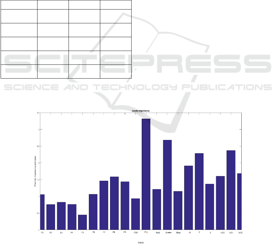
Figure 6: Bands contribution into the Random Forest segmentation.

In figure 6, the contribution of each band is

evaluated in the construction of the RF model with all

bands. The Green G, the Saturation S, and the

Saturation neighbours S15 are among those who

contribute the most but the highest contribution is

made by the F11 fluorescence band. This band

expresses the chlorophyll content of the plant as

described in (Gitelson et al., 1999), which explains

the high contribution of this band in the classification

of plant versus soil with no chlorophyll and algae and

moss with different chlorophyll composition. The

bands H15, S15 and V15 are also highly contributing

to the RF models constructions. These bands could

also be interpreted as noise reduced HSV signals, and

we can notice that the contribution of S15 was even

bigger than the contribution of S which indicates the

importance of its use.

4 CONCLUSIONS

As a conclusion, both used supervised machine

learning algorithms: SVM and RF approaches

succeeded to provide a useful tool for the plant

segmentation in the presence of challenging

background containing algae and moss. RF

approaches gave better results than the SVM

methods. The use of multiple bands showed that the

performance of the algorithms improves the

segmentation results especially with the SVM

models. Within the RF approach, bands contribution

to the final results vary and the highest contribution is

the ratio fluorescence which highlights the role of

these bands in such machine learning approaches. In

addition, the neighbourhood information introduced

by the channels H15, S15, and V15 contributed

considerably to the construction of the model and to

the improvement of the segmentation results.

One limitation of this approach is that it is based

on the expert knowledge constructing the data needed

for training the model (supervised machine learning).

In this sense, bad quality labelled image (a bad expert

segmentation) will result in a bad model for

segmentation.

To avoid this dependence, we will develop, in

future work, unsupervised models for the segmenta-

tion of the plants. Moreover, more features will be

included in the classification parameters such as

texture features to improve the segmentation results.

We will also focus on the plant 3D acquisition to

obtain more data (such as height and volume)

describing its responses to the environment (drought,

nutrients, biotic stress). These 3D information will

also be helpful for the segmentation and the time

tracking of individual plant leaves.

ACKNOWLEDGEMENTS

The authors thank Joke Belza for her help with the

manual segmentation of the data.

This work was financed by TIMESCALE, a

HORIZON 2020 project, and Ghent University.

REFERENCES

Arend D., Lange M., Pape J-M., Weigelt-Fischer K.,

Fernando Arana-Ceballos, Mücke I., Klukas C.,

Altmann T., Scholz U., and Junker A. 2016, “Data

Descriptor: Quantitative monitoring of Arabidopsis

thaliana growth and development using high-

throughput plant phenotyping”, Scientific Data 3,

Article number: 160055.

Åstrand B., and Johansson M. 2006; Segmentation of

partially occluded plant leaves; 13th International

Conference on Systems, Signals and Image Processing;

September 21-23, 2006, Budapest, Hungary.

Baker N. R. 2008, Chlorophyll Fluorescence: A Probe of

Photosynthesis In Vivo, Annual Review of Plant

Biology, 59:89-113.

Breiman L. 2001, “Random Forests”, Machine Learning,

pp 5–32, October 2001, Volume 45, Issue 1.

Cortes C., Vapnik V. 1995, “Support-Vector Networks”,

Machine Learning, 20, 273-297.

Gitelson A. A., Buschmann, C., and Lichtenthaler H. K.

1999; The Chlorophyll Fluorescence Ratio F735/F700

as an Accurate Measure of the Chlorophyll Content in

Plants, Remote Sensing Environment 69:296–302.

Navarro P. J., Pérez F., Weiss J., and Egea-Cortines M.

2016, “Machine Learning and Computer Vision System

for Phenotype Data Acquisition and Analysis in

Plants”, Sensors (Basel). 2016 May; 16(5): 641.

Scharr H., Minervini M., French A. P., Klukas Ch., Kramer

D. M., Liu X., Luengo I., Pape J-M., Polder G.,

Vukadinovic D., Yin X., and Tsaftaris S. A. 2016, “Leaf

segmentation in plant phenotyping: a collation study”,

Machine Vision and Applications 27:585–606.

De Vylder J., Vandenbussche F., Hu Y., Philips W., and

Van Der Straeten D. 2012, “Rosette Tracker: An Open

Source Image Analysis Tool for Automatic

Quantification of Genotype Effects.”, Plant Physiology,

November 2012, Vol. 160, pp. 1149–1159.