CRN: End-to-end Convolutional Recurrent Network Structure Applied
to Vehicle Classification
Mohamed Ilyes Lakhal
1
, Sergio Escalera
2
and Hakan Cevikalp
3
1
Queen Mary University of London, London, U.K.
2
University of Barcelona and Computer Vision Center UAB, Barcelona, Spain
3
Eskisehir Osmangazi University, Eskisehir, Turkey
Keywords:
Vehicle Classification, Deep Learning, End-to-end Learning.
Abstract:
Vehicle type classification is considered to be a central part of Intelligent Traffic Systems. In the recent years,
deep learning methods have emerged in as being the state-of-the-art in many computer vision tasks. In this
paper, we present a novel yet simple deep learning framework for the vehicle type classification problem. We
propose an end-to-end trainable system, that combines convolution neural network for feature extraction and
recurrent neural network as a classifier. The recurrent network structure is used to handle various types of
feature inputs, and at the same time allows to produce a single or a set of class predictions. In order to assess
the effectiveness of our solution, we have conducted a set of experiments in two public datasets, obtaining
state of the art results. In addition, we also report results on the newly released MIO-TCD dataset.
1 INTRODUCTION
The vehicle classification task is an important vision
problem, with applications to illegal vehicle type re-
cognition, traffic surveillance, and autonomous na-
vigation, among others. Traffic surveillance camera
systems are an essential component of an Intelligent
Traffic System. They include automatic monitoring
digital cameras that record high-resolution static ima-
ges of passing vehicles and other moving objects
(Tang et al., 2017). This source of information is
highly valuable for data mining and pattern classifica-
tion. Thus, a good procedure for classification is cru-
cial to this task. Classical machine learning tools do
not provide high performance solutions in this case.
On the other hand, deep learning techniques are the
current state-of-the-art in many Computer Vision and
Machine Learning problems. Following this trend,
we address the Vehicle type classification problem
by combining convolutional neural networks (CNNs)
structure with recurrent neural networks (RNNs). The
idea is simple and intuitive, and can be easily adapted
to other application scenarios, such as multi-label le-
arning, without any further additional structure. To
the best of our knowledge, this is the first attempt
that provides an end-to-end deep learning solution of
CNN and RNN to the vehicle classification task.
To summarize, the main contributions of our paper
are:
• Merging two deep learning models into a single
structure framework.
• Learning of rich high-dimensional feature vectors
in an end-to-end fashion.
• First attempt that uses such model to vehicle clas-
sification task, achieving state-of-the-art on two
datasets, and very competing results on a huge
real-world traffic surveillance dataset.
The rest of the paper is structured as following:
Section 2 provides a brief overview of the back-
ground literature on the topic, Section 3 describes our
CRN model, and the experimental results are given
in Section 4. Finally, we summarize our work with a
conclusion in Section 5.
2 RELATED WORK
Most of the vision-based methods for vehicle classi-
fication fall into two categories: model based met-
hods and appearance-based methods (Chen and El-
lis, 2011). In model based methods (Gupte et al.,
2002; Hsieh et al., 2006; Lai et al., 2001; Messelodi
et al., 2005; Zhang et al., 2012), geometric measure-
ments such as length, width, and height are used to
recover the vehicle’s 3D parameters. In (Nieto et al.,
2011), a 3D vehicle modeling has been proposed for
detection and classification by means of the integra-
tion of temporal information and model priors within
Lakhal, M., Escalera, S. and Cevikalp, H.
CRN: End-to-end Convolutional Recurrent Network Structure Applied to Vehicle Classification.
DOI: 10.5220/0006533601370144
In Proceedings of the 13th International Joint Conference on Computer Vision, Imaging and Computer Graphics Theory and Applications (VISIGRAPP 2018) - Volume 5: VISAPP, pages
137-144
ISBN: 978-989-758-290-5
Copyright © 2018 by SCITEPRESS – Science and Technology Publications, Lda. All rights reserved
137

Figure 1: Proposed CRN model. First, the three channels input image is processed through a series of convolutions and pool-
ing. Then, after reaching the fifth stage, we flatten the resulting set of features into a single high-dimensional representation
φ(I) ∈ R
f
. Finally, we feed the feature vector to the LSTM that learns the corresponding class label.
a Markov Chain Monte Carlo (MCMC). A 3D mo-
del, along with 3DHOG (which is an extension of
HOG (Dalal and Triggs, 2005) feature by applying
3D spatial modelling), has been successfully applied
to detect and classify vehicles (Buch et al., 2009).
The appearance-based methods (Hasegawa and Ka-
nade, 2005; Ma and Grimson, 2005; Zhang et al.,
2007) rely on the extraction of appearance features
(e.g., SIFT (Lowe, 2004), Sobel edges (Sobel, 1970))
from either frontal or side views of vehicle images to
classify them (Dong et al., 2014). A PCA-based, in-
tegrated vehicle classification framework is presented
in (Zhang et al., 2006). It consists of segmenting and
normalizing the vehicles from the input video stream,
after this step a PCA-based classifier (Eigenvehicle,
and PCA-SVM) is applied on the resulting segments.
In (Morris and Trivedi, 2006), the authors present
a tracking system with the ability to classify vehicles
into three classes. A 10-feature measurement vector
is extracted and its size is reduced by either princi-
pal component analysis (PCA) or linear discriminant
analysis (LDA), followed by a weighted K-nearest
neighbors (KNN) classifier. Another approach (Tang
et al., 2017) uses a more engineering solution cal-
led Local Gabor Binary Pattern Histogram Sequence
(Huang et al., 2011). In (Xiang et al., 2016), a sur-
veillance video based vehicle classification is presen-
ted. It uses local and structural features and sparse
coding; and multi-scale spatial max pooling is app-
lied to obtain more discriminative and representative
features.
More recently, deep learning approaches have
attracted the attention of various computer vision
tasks including the vehicle classification problem, and
many works have been proposed in this direction. In
(Zhou et al., 2016), two methods have been used; the
first one is fine tuning over the AlexNet (Krizhev-
sky et al., 2012) architecture, as for the second so-
lution the authors extracted features from the fully
connected layer of a pre-trained AlexNet on Image-
Net (Russakovsky et al., 2014), followed by an SVM
as a classifier. In (He et al., 2015), the authors con-
ducted a set of experiments to compare CNN features
against other type of feature descriptors, but the ex-
periments were conducted on a small subset of Ima-
geNet dataset. Moreover, semi-unsupervised Convo-
lutional Neural Network has been proposed in (Dong
et al., 2014). The weights of the network are learned
in an unsupervised manner via sparse filtering, while
the final classifier is trained in a supervised way using
the labeled dataset that was collected. The problem
with such pre-training is that it does not scale well
with large convolutional networks. In (Wang et al.,
2016) deep learning is also applied to Traffic Surveil-
lance Video problem. The authors first use CNN de-
tector to select region proposals, and then features are
obtained through a fully connected network. Finally
K-means is applied to cluster those proposals. In (Ji-
ang and Zhang, 2016), the authors proposed to use a
CNN for vehicle detection and recognition from video
stream in a weakly-supervised manner. Research on
multi-label classification using deep learning are also
conducted, e.g., the paper (Huo et al., 2016) presents
a Region-based CNN (RCNN) solution for vehicle re-
cognition problem.
In this paper, we present an appearance-based
vehicle type classification method. We combine CNN
and RNN into a single structure called CRN.
3 PROPOSED ARCHITECTURE
In this section, we describe the proposed CRN model.
The framework, offers a general way to approach the
vehicle classification problem. We also provide de-
tails of a typical implementation of such model, na-
med ESOGU. We will also highlight the importance
of feature learning part of this model.
3.1 CRN Model
Most of the successful deep learning models for
object recognition are built from stacking multiple
layers of convolutional operation and other operati-
ons such as batch normalization (Ioffe and Szegedy,
VISAPP 2018 - International Conference on Computer Vision Theory and Applications
138

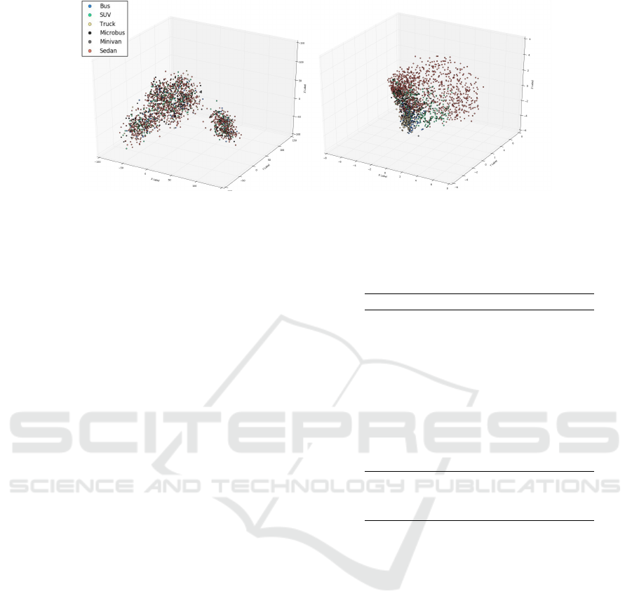
Figure 2: 3D scatter-plot of the features obtained from the test set of the BITVehicle dataset: (left) Pre-trained features; (right)
ESOGU features.
2015). Moreover, some recent works on image cap-
tioning (Vinyals et al., 2017; Xu et al., 2015) have
proven the effectiveness of the use of recurrent neu-
ral network as a pipeline for handling different type
of modalities (Vinyals et al., 2017). The idea is to
use features extracted from a pre-trained deep model.
For example, in (Vinyals et al., 2017) authors have
considered the use of GoogLeNet (Szegedy et al.,
2014). While CNNs are the state-of-the-art model
for image classification (He et al., 2016; Krizhevsky
et al., 2012; Simonyan and Zisserman, 2014; Szegedy
et al., 2014), we want to have a model that learns rich
high level features, and at the same time uses the flex-
ibility of the RNN network. This key observation is
our main motivation to our proposed solution. Our
CRN framework (see Figure 1), combines the convo-
lutional neural network with recurrent structure. This
allows the RNN to act as a classifier and the features
are learned in an ”end-to-end” fashion from the con-
volutional neural network. It also gives us a very flex-
ible framework to work with, i.e., the recurrent struc-
ture can handle variable length of inputs and produces
variable length of output too. As an example, to tackle
multi-label image classification (Li et al., 2014), the
RNN will learn to produce a sequence of labels wit-
hout any further structure or processing on the model.
Also, on the input side, depending on the application,
we can either consider working with a set of features
from the convolutional layer, or flatten the vector.
In this study, we propose two implementations of
the CRN framework: ESOGU, and ESOGU
f c
, where
the difference is only on the number of fully con-
nected layers. In the ESOGU model, we directly flat-
ten the last convolutional layer and give it as input
to the RNN. Whereas, in the ESOGU
f c
model, we
add extra fully connected layers to downsample the
dimensionality of our features. Details of the archi-
tecture of the later model are given in Table 1. The
images are re-scaled to 224 × 224 pixels, which serve
Table 1: ESOGU
f c
, implementation of the CRN model for
traffic vehicle classification. Where each ConvBlock, cor-
respond to the sequence ’Conv-Conv-ReLU-Pool’.
Module Layers Output Size
CNN
Conv [224 × 224]
Conv [224 × 224]
Pool [112 × 112]
ConvBlock
1
[56 × 56]
ConvBlock
2
[28 × 28]
ConvBlock
3
[14 × 14]
ConvBlock
4
[7 × 7]
FC
1
[25088]
FC
2
[4096]
FC
3
[4096]
RNN
LSTM nb
classes
as input to our model. After the convolution stage,
we flatten the last layer that will act as a feature des-
criptor of size 4096 for the ESOGU
f c
, and 25088 for
the ESOGU. Finally, we feed our descriptors to the
recurrent network that implements classification. In
this framework, we choose to work with LSTM (Ho-
chreiter and Schmidhuber, 1997).
3.2 Feature Learning
It is known that the performance of a classifier does
heavily depend on the choice of the feature represen-
tation (Bengio et al., 2013). In (Donahue et al., 2014),
the authors have shown that features extracted from
the activation of a convolutional network trained in a
fully supervised fashion can be in fact used as a gene-
ric descriptor. Empirical validations have been carried
out on small standard benchmark object recognition
tasks, including Caltech-101 (Fei-Fei et al., 2007).
In this study, we further investigate the use of deep
features as a generic descriptor for object classifica-
CRN: End-to-end Convolutional Recurrent Network Structure Applied to Vehicle Classification
139

tion task. Figure 2 shows 3D-PCA of features ex-
tracted from a pre-trained model on ImageNet (Deng
et al., 2009), and trained CRN model on the target set.
In the CRN model, when considering to work with
only the RNN part along with the learned features,
for small datasets the fully connected layer is a good
choice as feature extractor. However, in real world
large scale datasets, we argue that in fact the above
choice would not be appropriate due to the fact that
these images have a high range of geometric shapes
and illumination properties that could not be handled
by a small feature vector. We thus have to work with
other type of features, such as the upper level of con-
volution layers of a CNN. This idea was successfully
applied to other type of problems such like action re-
cognition (Sharma et al., 2015), where the authors use
pre-trained convolutional features and train an atten-
tion model.
As can be seen from our architecture, taking the
convolution layer without flattening as feature extrac-
tor is straighforward, since we would only have to
merge the last convolution layer with the RNN di-
rectly. To support our hypothesis, we conduct two
experiments on more realistic dataset, the MIO-TCD.
In the first one, features vectors are extracted directly
from a trained CRN model, and we train an RNN to
classify them. In the second experiment, convolutio-
nal features are obtained from the last convolutional
layer of pre-trained model on ImageNet (Deng et al.,
2009), and an attention based model is applied for
classification. We find that indeed, the second mo-
del performs way better than the one that uses only
one vector as feature input. These results confirm our
earlier hypothesis that claims: ”For the CRN model,
training a set of features when the dataset is large,
helps for better generalization”.
3.3 Loss Function
To train our model, we use the cross-entropy loss
function defined as follows:
L (X,Y ) = −
1
n
n
∑
i=1
[y
i
log( ˆy
i
) + (1 − y
i
)log(1 − ˆy
i
)].
where y
i
is the true label of the i-th sample, ˆy
i
is the
predicted class probabilities by the model, n the num-
ber of train samples, X the train set, and Y its corre-
sponding labels.
4 EXPERIMENTAL RESULTS
We have conducted a set of experiments on three da-
tasets: The Road vehicle dataset (Zhou et al., 2016),
(a) (b) (c) (d)
Figure 3: Images examples from the Vehicle classification
dataset: (a)-(b) Passenger; (c)-(d) Other.
Table 2: Results obtained on the Road vehicle dataset.
Method Acc
bal
Mean
Recall
Cohen
Kappa
Im-RNN 98.94% 98.94% 97.88%
ESOGU 97.92% 97.93% 95.76%
Fts-RNN 97.39% 97.39% 94.11%
(Zhou et al.,
2016)
97.35% − −
BIT-Vehicle (Dong et al., 2014), and the MIO-TCD
dataset. Because of the limited number of samples
on the first two datasets (Road vehicle dataset (Zhou
et al., 2016), BIT-Vehicle (Dong et al., 2014)), we ran
all the experiments using ESOGU model that has only
one fully connected layer of dimension 25088. The
two other models are, Fts-RNN and Im-RNN. In the
Fts-RNN model, we take vectors from the fully con-
nected layer of the ESOGU model as descriptors, and
the RNN is used as classifier. The other model, Im-
RNN uses RNN as a classifier on the features extrac-
ted by a pre-trained model (VGG-16 in this study).
For all the three benchmarks, we train the ESOGU,
and the ESOGU
f c
from scratch, i.e., we do not have
a pre-training phase on ImageNet. The experiments
were carried out on a machine equipped with 32 GB
of RAM, and an NVIDIA GTX 1080 with 8 GB GPU.
4.1 Metrics
To assess the proposed model, we use three metrics:
Accuracy,Mean Precision , Mean Recall , and Cohen
Kappa. Definitions are given below:
Accuracy =
T P + TN
T P + TN + FP + FN
(1)
Prec
i
=
T P
T P + FP
(2)
Rec
i
=
T P
T P + FN
(3)
MeanPrecision =
C
∑
i=1
Prec
i
, (4)
MeanRecall =
C
∑
i=1
Rec
i
, (5)
VISAPP 2018 - International Conference on Computer Vision Theory and Applications
140

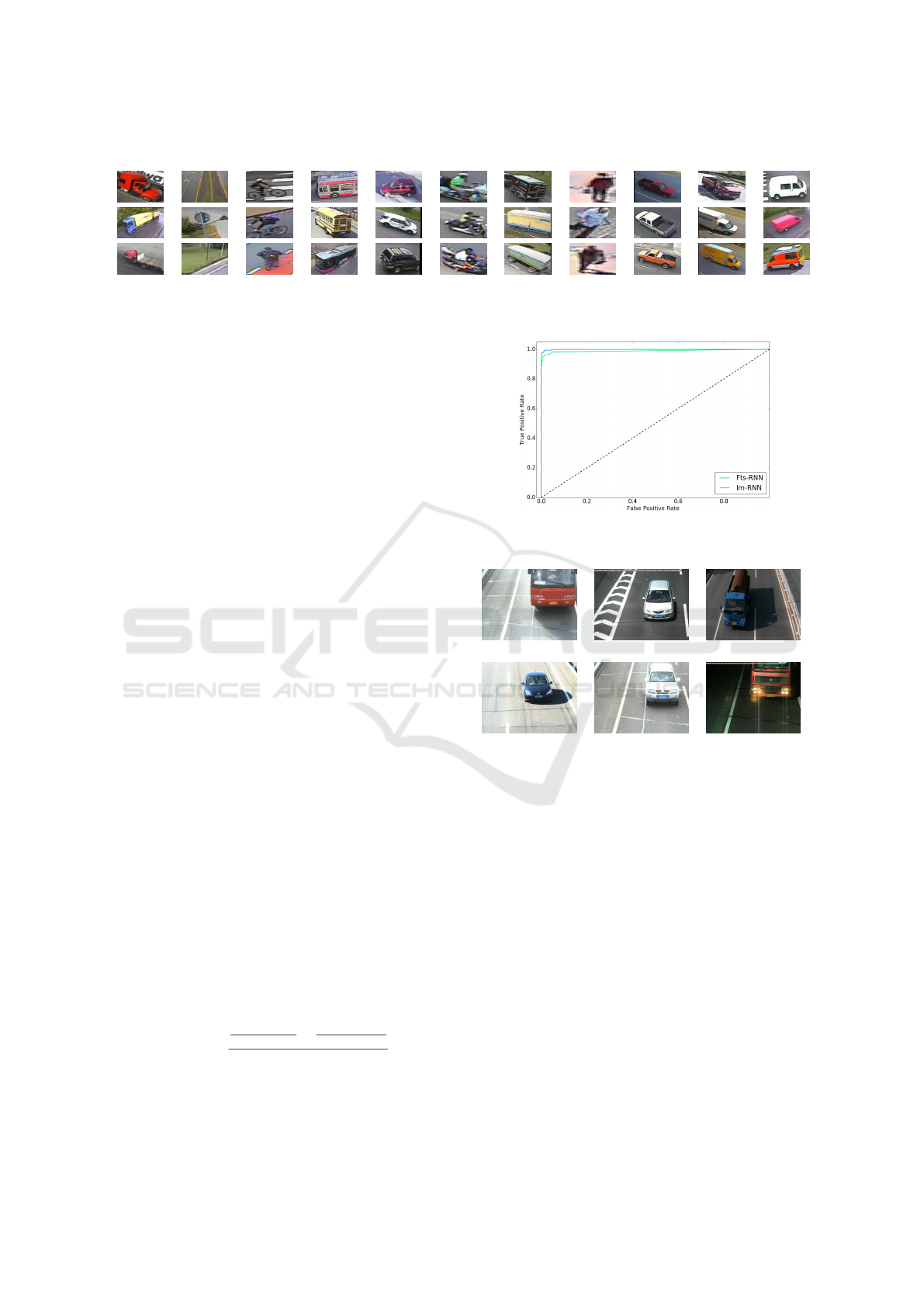
(a) (b) (c) (d) (e) (f) (g) (h) (i) (j) (k)
Figure 4: Samples from the MIO-TCD: (a) Articulated truck; (b) Background; (c) Bicycle; (d) Bus; (e) Car; (f) Motorcycle;
(g) Non-motorized vehicle; (h) Pedestrian; (i) Pickup truck; (j) Single unit truck; (k) Work van.
where T P is true positives, FN false negatives, T N
true negatives, FP false positives, Rec
i
is the per-class
recall, and C is the total number of classes.
Cohen kappa (Cohen, 1960), is a statistic that me-
asures inter-annotator agreement as defined in Equa-
tion 6, where p
o
is the empirical probability of
agreement with the label assigned to any sample, and
p
e
is the expected agreement when both annotators
assign labels randomly.
κ = (p
o
− p
e
)/(1 − p
e
) (6)
This function is used on a classification problem, and
the obtained scores express the level of agreement be-
tween two annotators.
4.2 Road Vehicle Dataset
The Road vehicle dataset (Zhou et al., 2016) (see Fi-
gure 3) contains images that are taken from a sta-
tic camera along an express way. The original da-
taset contains 300 images of vehicles on multiple la-
nes, after some pre-processing, 983 images are obtai-
ned. Among these, 940 are valid images, i.e., image
that contains a whole vehicle, and 43 invalid ima-
ges, where most of them contain overlapping vehi-
cles. The dataset can be used for either vehicle de-
tection or classification. For the classification task,
there are two classes: passenger class and other class.
The passenger class includes: SUV, and MPV, whe-
reas the other class contains: van, truck, and other
types of vehicle. After doing some initial processing,
i.e., croping and segmentation, the classification da-
taset contains 1,442 images for the passenger class,
and 985 for other class.
In order to evaluate our model with other state-of-
the-art methods, we employ the same metric defined
in Equation 7 as suggested in (Zhou et al., 2016):
Acc
bal
=
Correct(pass)
Size(pass)
+
Correct(other)
Size(other)
2
(7)
where Correct(pass) represents the number of correct
predictions in passenger class, and Size(pass) is its
size.
Figure 5: ROC over the test set for the Road vehicle dataset.
(a) (b) (c)
(d) (e) (f)
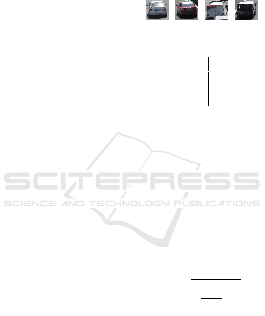
Figure 6: Samples from the BITVehicle dataset: (a) Bus;
(b) Microbus; (c) Minivan; (d) Sedan; (e) SUV; (f) Truck.
The test results are shown in Table 2. The perfor-
mance of the ESOGU was slightly below the Im-RNN
model. This is explained by the fact that the used da-
taset is fairly small, and we did not consider data aug-
mentation. Figure 5 shows the ROC for the Im-RNN
and Fts-RNN models. Another remark here is that,
due to the limited train/set samples, the results are in
general close to each other.
4.3 BIT-Vehicle
The BIT-Vehicle (Dong et al., 2014) is a classification
dataset that contains 900 vehicles images divided into
six categories: Bus, Microbus, Minivan, Sedan, SUV,
and Truck (see Figure 6). Each category contains 150
image samples of either 1600×1200, or 1920 × 1080
pixel size. The images contain changes in illumina-
tion condition, scale, the surface color of vehicles and
CRN: End-to-end Convolutional Recurrent Network Structure Applied to Vehicle Classification
141

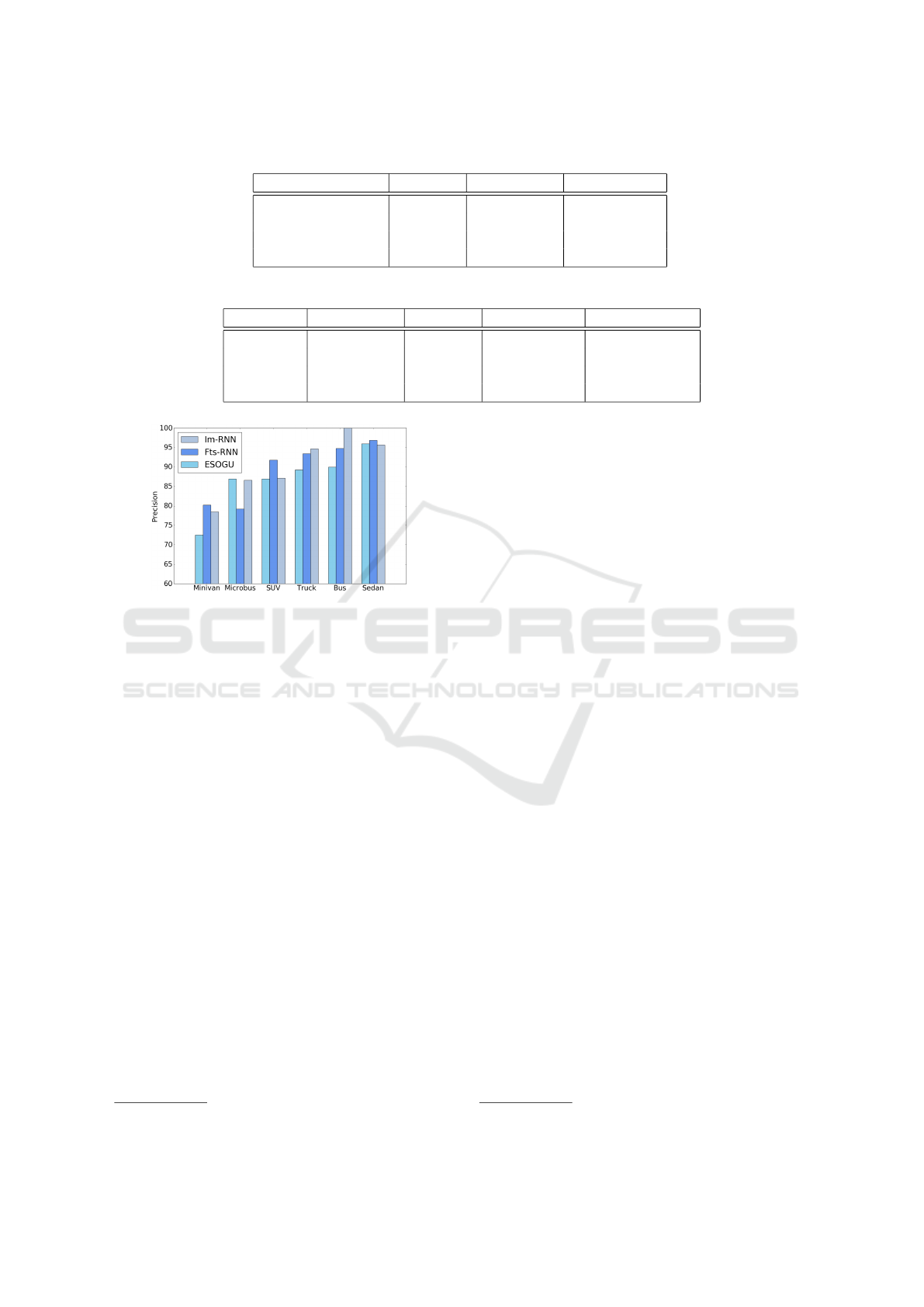
Table 3: Models results over the BITVehicle test set.
Method Accuracy Mean Recall Cohen Kappa
Fts-RNN 93.40% 88.01% 89.16%
Im-RNN 93.20% 88.73% 88.74%
(Dong et al., 2014) 92.89% - −
ESOGU 92.08% 86.18% 86.95%
Table 4: Classification results on the MIO-TCD challenge.
Method Mean Recall Accuracy Cohen Kappa Mean Precision
VGG16
FT
85.02% 96.16% 94.03% 88.02%
ESOGU
f c
84.77% 93.62% 90.24% 79.37%
ESOGU 83.86% 93.74% 90.37% 77.72%
AlexNet 75.83% 93.30% 89.57% 77.29%
Figure 7: Per-class precision for the three described models
on the BITVehicle dataset.
viewpoint. This dataset was captured at different pla-
ces and different times.
In this dataset, our three models generalize well
on the test set. In Table 3 we give the accuracy, mean
accuracy, and the Cohen Kappa score. Figure 7 shows
the per-class precision of each model. Again, the ge-
neral performance of the presented solutions are simi-
lar.
4.4 MIO-TCD Dataset
The MIO-TCD dataset
1
consists of total 786,702
images with 648,959 in the classification dataset and
137,743 in the localization dataset acquired at diffe-
rent times of the day and different periods of the year
by thousands of traffic cameras deployed all over Ca-
nada and the United States. The dataset is divided in
two parts, the ”classification dataset” and the ”locali-
zation dataset”. For the classification task, the dataset
is divided into 11 classes as shown in Figure 4.
It is worth noticing that for the classification task, the
original set is highly unbalanced, that is, the class
samples are not equally distributed. For example,
there are 260,518 samples for the highest class (car
class), and 1, 751 examples for the under-represented
1
http://podoce.dinf.usherbrooke.ca/challenge/dataset/
one (non-motorized vehicle class). So, if we feed di-
rectly the dataset as it is to our classifier, we would
learn only models of classes that have the largest num-
ber training samples. To overcome this, we use data
augmentation (Krizhevsky et al., 2012) only on under-
represented classes in order to have more data exam-
ples for the training phase. Also, for each epoch we
get random samples per class of fixed size as shown
below:
Batch[class
i
] = {z
i j
|z
i j
∼ R(X
i
);1 ≤ i ≤ C;1 ≤ j ≤ m}
Here, we denote by z
i j
the randomly chosen element,
R(.) the distribution that returns an element from a
set, where each element has the same proportion to be
chosen, C the number of classes (11 in our case), and
m is a fixed integer which represents the size of each
class per epoch.
Table 4 shows our results comparing to some of
the submissions. We refer the reader to the official
ranking for complete comparison.
2
Here we de-
note by VGG16
FT
, the fine tuned VGG16. Our met-
hod was able to achieve a competing results, with a
good generalization to unseen challenging and realis-
tic data.
5 CONCLUSIONS
We have introduced a simple yet robust deep architec-
ture for the vehicle classification problem. Our solu-
tion differs from the other state-of-the art in the sense
that we propose to use the recurrent neural network as
a classifier, and the feature learning part is performed
using a CNN. The whole system is trained in end-to-
end manner. We have demonstrated the use of deep
feature as a proper choice for representation. We fi-
nally suggested an extension of this framework when
2
http://podoce.dinf.usherbrooke.ca/results/classification
VISAPP 2018 - International Conference on Computer Vision Theory and Applications
142

dealing with more challenging dataset and supported
it with further experiments. The extension is to use M
feature vectors of size p as input to the recurrent struc-
ture instead of one feature vector. The proposed fra-
mework can easily adapt itself to other scenarios like
multi-label image classification without adding extra
layers to the network architecture.
ACKNOWLEDGEMENTS
This work has been partially supported by the Spa-
nish project TIN2016-74946-P (MINECO/FEDER,
UE) and CERCA Programme / Generalitat de Cata-
lunya.
REFERENCES
Bengio, Y., Courville, A., and Vincent, P. (2013). Represen-
tation learning: A review and new perspectives. IEEE
Trans. Pattern Anal. Mach. Intell., 35(8):1798–1828.
Buch, N., Orwell, J., and Velastin, S. A. (2009). 3d extended
histogram of oriented gradients (3dhog) for classifica-
tion of road users in urban scenes. In Proceedings of
the British Machine Vision Conference, pages 15.1–
15.11. BMVA Press. doi:10.5244/C.23.15.
Chen, Z. and Ellis, T. (2011). Multi-shape descriptor vehi-
cle classification for urban traffic. In 2011 Internatio-
nal Conference on Digital Image Computing: Techni-
ques and Applications, pages 456–461.
Cohen, J. (1960). A coefficient of agreement for nominal
scales. Educational and Psychological Measurement,
20(1):37–46.
Dalal, N. and Triggs, B. (2005). Histograms of oriented
gradients for human detection. In Proceedings of the
2005 IEEE Computer Society Conference on Compu-
ter Vision and Pattern Recognition (CVPR’05) - Vo-
lume 1 - Volume 01, CVPR ’05, pages 886–893, Wa-
shington, DC, USA. IEEE Computer Society.
Deng, J., Dong, W., Socher, R., Li, L.-J., Li, K., and Fei-
Fei, L. (2009). ImageNet: A Large-Scale Hierarchical
Image Database. In CVPR09.
Donahue, J., Jia, Y., Vinyals, O., Hoffman, J., Zhang, N.,
Tzeng, E., and Darrell, T. (2014). Decaf: A deep con-
volutional activation feature for generic visual recog-
nition. In International Conference in Machine Lear-
ning (ICML).
Dong, Z., Pei, M., He, Y., Liu, T., Dong, Y., and Jia, Y.
(2014). Vehicle type classification using unsupervi-
sed convolutional neural network. In 2014 22nd In-
ternational Conference on Pattern Recognition, pages
172–177.
Fei-Fei, L., Fergus, R., and Perona, P. (2007). Lear-
ning generative visual models from few training ex-
amples: An incremental bayesian approach tested on
101 object categories. Comput. Vis. Image Underst.,
106(1):59–70.
Gupte, S., Masoud, O., Martin, R. F., and Papanikolopou-
los, N. P. (2002). Detection and classification of vehi-
cles. Trans. Intell. Transport. Sys., 3(1):37–47.
Hasegawa, O. and Kanade, T. (2005). Type classification,
color estimation, and specific target detection of mo-
ving targets on public streets. Machine Vision and Ap-
plications, 16(2):116–121.
He, D., Lang, C., Feng, S., Du, X., and Zhang, C. (2015).
Vehicle detection and classification based on convolu-
tional neural network. In Proceedings of the 7th In-
ternational Conference on Internet Multimedia Com-
puting and Service, ICIMCS ’15, pages 3:1–3:5, New
York, NY, USA. ACM.
He, K., Zhang, X., Ren, S., and Sun, J. (2016). Deep re-
sidual learning for image recognition. In The IEEE
Conference on Computer Vision and Pattern Recogni-
tion (CVPR).
Hochreiter, S. and Schmidhuber, J. (1997). Long short-term
memory. Neural Comput., 9(8):1735–1780.
Hsieh, J.-W., Yu, S.-H., Chen, Y.-S., and Hu, W.-F.
(2006). Automatic traffic surveillance system for vehi-
cle tracking and classification. IEEE Transactions on
Intelligent Transportation Systems, 7(2):175–187.
Huang, D., Shan, C., Ardabilian, M., Wang, Y., and Chen,
L. (2011). Local binary patterns and its application to
facial image analysis: A survey. IEEE Transactions on
Systems, Man, and Cybernetics, Part C (Applications
and Reviews), 41(6):765–781.
Huo, Z., Xia, Y., and Zhang, B. (2016). Vehicle type classi-
fication and attribute prediction using multi-task rcnn.
In 2016 9th International Congress on Image and Sig-
nal Processing, BioMedical Engineering and Infor-
matics (CISP-BMEI), pages 564–569.
Ioffe, S. and Szegedy, C. (2015). Batch normalization:
Accelerating deep network training by reducing in-
ternal covariate shift. In Proceedings of the 32nd In-
ternational Conference on Machine Learning, ICML
2015, Lille, France, 6-11 July 2015, pages 448–456.
Jiang, C. and Zhang, B. (2016). Weakly-supervised vehi-
cle detection and classification by convolutional neu-
ral network. In 2016 9th International Congress on
Image and Signal Processing, BioMedical Engineer-
ing and Informatics (CISP-BMEI), pages 570–575.
Krizhevsky, A., Sutskever, I., and Hinton, G. E. (2012).
Imagenet classification with deep convolutional neu-
ral networks. In Pereira, F., Burges, C. J. C., Bottou,
L., and Weinberger, K. Q., editors, Advances in Neu-
ral Information Processing Systems 25, pages 1097–
1105. Curran Associates, Inc.
Lai, A. H. S., Fung, G. S. K., and Yung, N. H. C.
(2001). Vehicle type classification from visual-based
dimension estimation. In ITSC 2001. 2001 IEEE In-
telligent Transportation Systems. Proceedings (Cat.
No.01TH8585), pages 201–206.
Li, X., Zhao, F., and Guo, Y. (2014). Multi-label image
classification with a probabilistic label enhancement
model. In Proceedings of the Thirtieth Conference on
Uncertainty in Artificial Intelligence, UAI’14, pages
430–439, Arlington, Virginia, United States. AUAI
Press.
CRN: End-to-end Convolutional Recurrent Network Structure Applied to Vehicle Classification
143

Lowe, D. G. (2004). Distinctive image features from scale-
invariant keypoints. Int. J. Comput. Vision, 60(2):91–
110.
Ma, X. and Grimson, W. E. L. (2005). Edge-based rich
representation for vehicle classification. In Tenth
IEEE International Conference on Computer Vision
(ICCV’05) Volume 1, volume 2, pages 1185–1192 Vol.
2.
Messelodi, S., Modena, M., and Zanin, M. (2005). A com-
puter vision system for the detection and classification
of vehicles at urban road intersections. Pattern Anal.
Appl., 8(1):17–31.
Morris, B. and Trivedi, M. (2006). Improved vehicle clas-
sification in long traffic video by cooperating tracker
and classifier modules. In 2006 IEEE International
Conference on Video and Signal Based Surveillance,
pages 9–9.
Nieto, M., Unzueta, L., Cortes, A., Barandiaran, J., Otaegui,
O., and Sanchez, P. (2011). Real-time 3d modeling of
vehicles in low-cost mono camera systems. In Proc.
Int. Conf. on Computer Vision Theory and Applicati-
ons VISAPP, pages 459–464.
Russakovsky, O., Deng, J., Su, H., Krause, J., Satheesh, S.,
Ma, S., Huang, Z., Karpathy, A., Khosla, A., Bern-
stein, M. S., Berg, A. C., and Li, F. (2014). Image-
net large scale visual recognition challenge. CoRR,
abs/1409.0575.
Sharma, S., Kiros, R., and Salakhutdinov, R. (2015).
Action recognition using visual attention. CoRR,
abs/1511.04119.
Simonyan, K. and Zisserman, A. (2014). Very deep con-
volutional networks for large-scale image recognition.
CoRR, abs/1409.1556.
Sobel, I. E. (1970). Camera Models and Machine Percep-
tion. PhD thesis, Stanford, CA, USA. AAI7102831.
Szegedy, C., Liu, W., Jia, Y., Sermanet, P., Reed, S. E., An-
guelov, D., Erhan, D., Vanhoucke, V., and Rabinovich,
A. (2014). Going deeper with convolutions. CoRR,
abs/1409.4842.
Tang, Y., Zhang, C., Gu, R., Li, P., and Yang, B. (2017).
Vehicle detection and recognition for intelligent traffic
surveillance system. Multimedia Tools and Applicati-
ons, 76(4):5817–5832.
Vinyals, O., Toshev, A., Bengio, S., and Erhan, D.
(2017). Show and tell: Lessons learned from the 2015
MSCOCO image captioning challenge. IEEE Trans.
Pattern Anal. Mach. Intell., 39(4):652–663.
Wang, S., Liu, F., Gan, Z., and Cui, Z. (2016). Vehicle type
classification via adaptive feature clustering for traffic
surveillance video. In 2016 8th International Confe-
rence on Wireless Communications Signal Processing
(WCSP), pages 1–5.
Xiang, Z. Q., Huang, X. L., and Zou, Y. X. (2016). An
effective and robust multi-view vehicle classification
method based on local and structural features. In 2016
IEEE Second International Conference on Multimedia
Big Data (BigMM), pages 68–73.
Xu, K., Ba, J., Kiros, R., Cho, K., Courville, A., Salakhu-
dinov, R., Zemel, R., and Bengio, Y. (2015). Show,
attend and tell: Neural image caption generation with
visual attention. In Blei, D. and Bach, F., editors, Pro-
ceedings of the 32nd International Conference on Ma-
chine Learning (ICML-15), pages 2048–2057. JMLR
Workshop and Conference Proceedings.
Zhang, C., Chen, X., and bang Chen, W. (2006). A pca-
based vehicle classification framework. In 22nd Inter-
national Conference on Data Engineering Workshops
(ICDEW’06), pages 17–17.
Zhang, L., Li, S. Z., Yuan, X., and Xiang, S. (2007). Real-
time object classification in video surveillance based
on appearance learning. In 2007 IEEE Conference on
Computer Vision and Pattern Recognition, pages 1–8.
Zhang, Z., Tan, T., Huang, K., and Wang, Y. (2012).
Three-dimensional deformable-model-based localiza-
tion and recognition of road vehicles. IEEE Transacti-
ons on Image Processing, 21(1):1–13.
Zhou, Y., Nejati, H., Do, T. T., Cheung, N. M., and Cheah,
L. (2016). Image-based vehicle analysis using deep
neural network: A systematic study. In 2016 IEEE In-
ternational Conference on Digital Signal Processing
(DSP), pages 276–280.
VISAPP 2018 - International Conference on Computer Vision Theory and Applications
144