Omnidirectional Visual Odometry for Flying Robots

using Low-power Hardware

Simon Reich, Maurice Seer, Lars Berscheid, Florentin W

org

otter and Jan-Matthias Braun

Third Institute of Physics - Biophysics, Georg-August-Universit

at G

ottingen,

Friedrich-Hund-Platz 1, 37077 G

ottingen, Germany

Keywords:

Visual Odometry, Embedded Hardware, Omnidirectional Vision.

Abstract:

Currently, ﬂying robotic systems are in development for package delivery, aerial exploration in catastrophe areas,

or maintenance tasks. While many ﬂying robots are used in connection with powerful, stationary computing

systems, the challenge in autonomous devices—especially in indoor-rescue or rural missions—lies in the need

to do all processing internally on low power hardware. Furthermore, the device cannot rely on a well ordered or

marked surrounding. These requirements make computer vision an important and challenging task for such

systems. To cope with the cumulative problems of low frame rates in combination with high movement rates of

the aerial device, a hyperbolic mirror is mounted on top of a quadrocopter, recording omnidirectional images,

which can capture features during fast pose changes. The viability of this approach will be demonstrated by

analysing several scenes. Here, we present a novel autonomous robot, which performs all computations online

on low power embedded hardware and is therefore a truly autonomous robot. Furthermore, we introduce several

novel algorithms, which have a low computational complexity and therefore enable us to refrain from external

resources.

1 INTRODUCTION

Real time computer vision in fast moving robots re-

mains still a very challenging task, especially when

forced to use limited computing power, e.g. when

having to use embedded systems. There are several

robotic applications existing where this is needed and

one of the most challenging is visual guided on-board-

computed indoor ﬂight. There are no GPS signals

available and the autonomous aerial vehicle (AAV)

has to navigate quickly in often conﬁned spaces. To

enable collision detection, onboard sensors must be uti-

lized. The probably most prominent autonomous robot

is the unmanned car Stanley, which won the DARPA

Grand Challenge in 2005 (Thrun et al., 2006). Stanley

has a wide range of different sensors, including GPS,

laser range sensors, and RADAR sensors: The total po-

wer consumption accumulates to 500 W (Thrun et al.,

2006).

In recent years, energy efﬁcient hardware, which

is still powerful enough, and batteries, which offer

enough power, became available. This allowed on the

one hand for smaller robots and on the other hand for

complex motor control tasks and sensor evaluation—

as it is required in quadrocopters. However, active

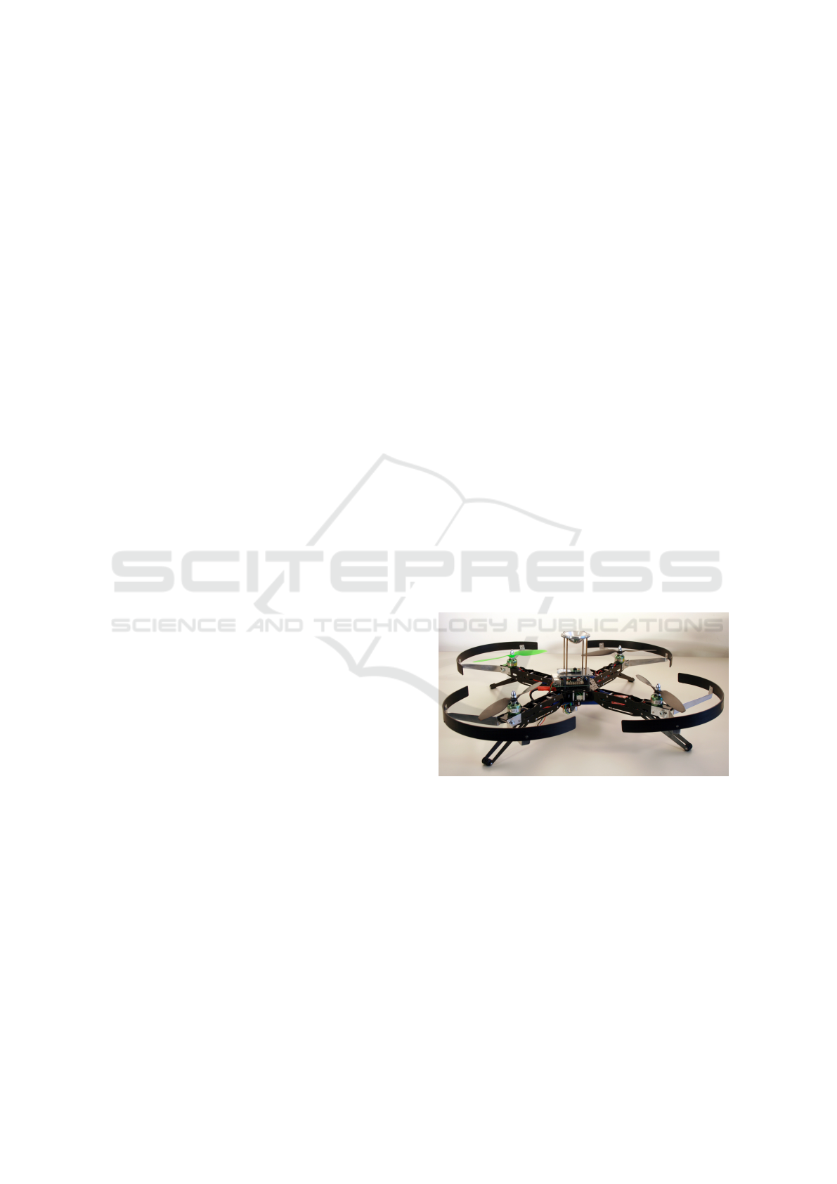
Figure 1: The quadrocopter utilized in this work. In the

center, a camera captures omnidirectional images via the

mounted mirror (Compare Fig. 3a).

sensors approaches often lack in high power require-

ments and heavy weight. Both problems are solved by

using an RGB camera, which is a passive sensor and

has low power consumption.

Previous work on autonomous ﬂight can be cate-

gorized into two research areas. First, a lot of works

focus on agile and accurate motion control. Most

prominent is the quadrocopter swarm of ETH Zurich,

which is able to perform synchronized dancing mo-

tions (Sch

ollig et al., 2012) or even to build simple

architectural structures (Augugliaro et al., 2014). But

Reich, S., Seer, M., Berscheid, L., Wörgötter, F. and Braun, J-M.

Omnidirectional Visual Odometry for Flying Robots using Low-power Hardware.

DOI: 10.5220/0006509704990507

In Proceedings of the 13th International Joint Conference on Computer Vision, Imaging and Computer Graphics Theory and Applications (VISIGRAPP 2018) - Volume 5: VISAPP, pages

499-507

ISBN: 978-989-758-290-5

499

these complex tasks heavily rely on external tracking

of the robots and are thus restricted to lab use. In anot-

her approach, artiﬁcial markers in the environment

simplify pose estimation (Eberli et al., 2011). For GPS

enabled areas, complete commercial solutions exist,

e.g. (Remes et al., 2013; Anai et al., 2012).

Second, there are approaches, which only use on-

line sensors for self localization. Still, in many studies

the computational expensive tasks are performed on

external hardware via Bluetooth or wireless LAN links,

e.g. (Engel et al., 2014; Teuli

ere et al., 2010), which

limit the independence of the devices. In recent years,

the miniaturization of computers and advancement in

battery design, driven mostly by rapid cell phone de-

velopment, has made it possible to build smaller auto-

nomous robots and perform computations in real time

on the AAV itself. While online computations result

in maximum autonomy, even today, real time compu-

tations on 3D data remain a complex task. Instead of

3D sensors as LIDAR, the Asus Xtion Pro, or the Mi-

crosoft Kinect sensor, most systems use a monocular

camera and perform 3D reconstruction.

For example, already in 2010 in (Olivares-M

endez

et al., 2010) detection of a planar landing zone for a

helicopter using a monocular camera is described, al-

lowing for autonomous landing of a helicopter. (Mori

and Scherer, 2013) use a front facing camera to detect

objects in the ﬂight path and estimate size. Yet, all

approaches with camera in a speciﬁc direction face the

problem of a small observation window.

Omnidirectional monocular cameras, which pro-

vide a 360

◦

view of the environment, have been

successfully applied to these problems. In (Gaspar

et al., 2001), a slow moving robot estimates the depth

of edges in a corridor using an omnidirectional camera.

(Rodr

ıguez-Canosa et al., 2012) apply this procedure

to an unstable ﬂying robot; however, no quantitative

results are shown. In (Demonceaux et al., 2006) this

method is shown to be able to achieve attitude measu-

rements.

In this work, we focus on navigating a ﬂying robot

in unknown, GPS-denied, indoor scenarios. All com-

putations are performed online and in real time—there

will be no external tracking. We ask: what is needed

to safely (and therefore reliably) detect features on a

hardware platform that very strongly jerks, jolts, and

may even ﬂip? And—if those can be found—how

to track them and use them for trajectory planning

on limited hardware in real time? One goal is to im-

prove navigation by introducing a novel lightweight

omnidirectional camera setup for embedded computer

systems. Lastly, we aim to extract features, track them

over multiple frames, compute a 3D point cloud, and

perform high level navigation tasks on this internal

model of the AAV’s environment.

In the following section, we shortly introduce our

hardware approach, a quadrocopter holding an omnidi-

rectional camera. Afterwards, the utilized algorithms

are shown. Then, we describe our experiments and

results, followed by a detailed discussion and conclu-

sion.

2 METHOD

This section divides into three parts: In 2.1 the har-

dware setup is presented, and in 2.2 our algorithms

to arrive at safe trajectory planning are shown. Las-

tly, we will discuss brieﬂy the theoretical limit of the

algorithms.

2.1 Hardware Setup

The hardware setup is depicted in Fig. 1: A quadro-

copter, controlled by a Raspberry Pi mini computer.

These robots are able to turn and even ﬂip on very

short notice. This poses the problem that a front facing

camera is not able to reliably track features, as it has

to deal with huge offsets and many features leaving

the camera’s ﬁeld of view. We therefore attached a

monocular camera pointing upwards on a hyperboli-

cally shaped mirror, which can also be replaced with

a spherical shaped mirror. Later, we will discuss the

advantages and disadvantages of these shapes. The

camera photographs with a resolution of 320x320 px

at a frequency of 30 Hz.

Additionally, we use an accelerometer and gy-

roscope as input. Also, any contemporary Bluetooth

gaming controller can be attached. This allows easy

control of high level features, e.g. issue the start or lan-

ding command. The 6D pose from the visual odometry

algorithm is merged with data from an accelerometer

and a gyroscope using a Kalman ﬁlter. All software

components run as modular and parallel nodes using

the Robot Operating System (ROS (Quigley et al.,

2009)).

2.2 Algorithms

In this section, we describe how we estimate the AAV’s

pose from an omnidirectional monocular RGB images.

All software components run as parallel nodes using

the Robot Operating System (ROS (Quigley et al.,

2009)).

An overview of the proposed system is given in

Fig. 2. First, we compute features and the optical ﬂow

based on the raw camera image. Dewarping the image

enables us to estimate the pose change from the last

VISAPP 2018 - International Conference on Computer Vision Theory and Applications

500

a) Compute features

and optical ﬂow

b) Dewarp &

compute 6 DoF pose

6 DoF

IMU

6 DoF

EKF

c) Fuse VO and

IMU via EKF

d) Compute depth

via triangulation

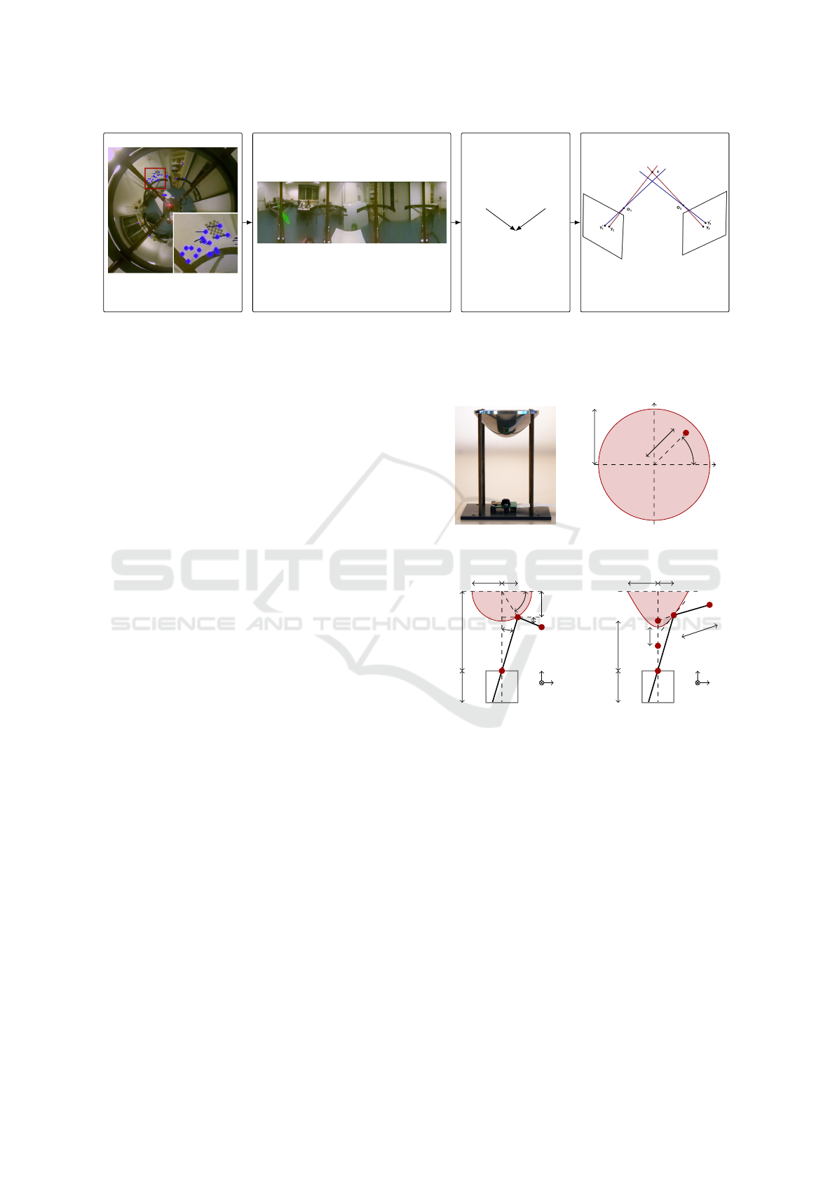
Figure 2: Pipeline of our proposed algorithm. a) Based on features we compute the optical ﬂow. b) After dewarping the image,

we estimate the pose change. c) An Extended Kalman Filter (EKF) combines the Visual Odometry (VO) results with values

from the Inertial Measurement Unit (IMU). d) After having tracked features for multiple frames, we can estimate the point’s

depth using triangulation and build a depth map.

camera frame (Fig. 2b). An Extended Kalman Fil-

ter (EKF) (Kalman, 1960) fuses the visual odometry

6 DoF results with the 6 DoF of the Inertial Measu-

rement Unit (Fig. 2c). Afterwards, a PID controller,

as demonstrated by (

Astr

om and H

agglund, 2006),

adjusts the motor controllers to manipulate the qua-

drocopter into the goal pose (which is deﬁned by e.g.

SLAM (Williams et al., 2009), corridor ﬂight algo-

rithms (Lange et al., 2012), etc.). As we keep a list of

all tracked features and their relative position to the

robot, we can triangulate each feature and compute

a depth estimate for each feature (Fig. 2d). This can

be used by high level algorithms for map building or

navigation tasks.

2.2.1 Feature Set

As already mentioned, we ﬁrst compute features on

the raw camera image. Features are points in an image,

which are easy to ﬁnd, recognize, and track in con-

secutive frames—usually areas rich in texture. Af-

terwards, we compute the optical ﬂow on these fea-

tures. There are numerous publications comparing

different feature algorithms—the most prominent algo-

rithms include FAST (Rosten and Drummond, 2006),

GFTT (Shi and Tomasi, 1994), ORB (Rublee et al.,

2011), SIFT (Lowe, 1999), and SURF (Bay et al.,

2006). Here, we use FAST as it offers a good FAST

offers the best trade-off between computational com-

plexity and quality of found features. This result is

not surprising, as FAST is known to be faster but also

ﬁnds less features (El-gayar et al., 2013; Heinly et al.,

2012).

2.2.2 Transformations between Image and

World Coordinates

In the following, we derive transformations

S,H

from

image space to the external frame of reference and

(a) The hyperbola mirror.

−φ

(b) Camera view of the mir-

ror.

2ε

(d) Side view of hyperbola

mirror.

Figure 3: Sketch of a camera observing an object

, which

appears at position

in the image plane (bottom left). The

top left ﬁgure depicts a simple pinhole model; on the top

right the camera is pointed at a spherical mirror and at the

bottom right at a hyperbolic mirror.

their inverse

−1

S,H

indicates a spherical and

a hy-

perbola shaped mirror. We denote object positions in

image space by 2D coordinates

in cartesian

)

or polar coordinates

(ρ,φ)

. We denote their counter-

parts in the external frame of reference as

~o ∈ R

. The

robot’s pose in the external frame of reference is de-

termined by its position

and orientation

: This is

the pose of the camera’s view as shown in Fig. 3c and

3d. As the derivation of the transformation includes

several coordinate system changes, we here present

the transformations.

Omnidirectional Visual Odometry for Flying Robots using Low-power Hardware

501

Spherical Mirror Model.

A spherical mirror is

mounted with its center in distance

above the ca-

mera (Fig. 3c). Using the real sphere radius

and

radius

in image space (Fig. 3b), the reﬂection’s po-

sition on the mirror can be computed independently

of camera parameters using the scaling factor

s =

With the unit vector

pointing from the reﬂection on

the mirror towards the object’s position ~o

(~o

) =





cosβcosφ

cosβsinφ

−sinβ





given the distance

h =

−ρ

, the angles

in Fig. 3b derived from the image coordinates, and

the rotation matrix

R(~q)

between the external frame

of reference and the camera system in Fig. 3b, we can

compute the position ~o by:

:~o

7−→~o :~o =~c+R(~q)





l −h(~o

)

+ d~e

(~o

)





For the inverse transformation

−1

, we use polar coor-

dinates:

−1

: ~o 7−→~o

: ~o

= r

cosα(~o) ·



cosφ(~o)

sinφ(~o)



with

φ = −atan2



−1

(~q)(~o −~c))

,(R

−1

(~q)(~o −~c))



and

= r

cosα(~o)

. As there is no explicit form for

cosα, we use the iterative approximation

cosα ≈



−sinα



·tan



arctan



−sinα −∆ sin β

r cos α



−2α +



for small focal lengths (

l − f ≈ l

) and large depths

(

 1).

Still, the solution is nontrivial and computational

expensive. Considering that we are using autonomous

robots, which perform all computations online on li-

mited hardware, this poses a problem.

Hyperbolic Mirror Model.

Using a hyperbola, the

inverse function can be computed easier and thus faster.

The surface of a hyperbolic mirror is deﬁned by

−

= 1 , a, b ∈ R (1)

with the semi-major axis

. The focal points

1,2

are

set apart by

√

+ b

=: 2ε

(Fig. 3d). The robot’s

position is deﬁned by the point in the middle of these

two focal points. The camera’s focal point coincides

with

. With

being the unit vector pointing from the

reﬂection on the mirror towards the object’s position

~o:

(~o

) =



s~o

,s~o

+ b

−ε







s~o

,s~o

+ b

−ε





the transformation T

:~o

7−→~o :

~o =~c + R(~q)





ρ(~o

)

+ b

+ d~e

(~o

)





and therefore the object position at a distance

is de-

ﬁned as

~o =~r + R



~o + d~e



. For the inverse transfor-

mation in polar coordinates as for the spherical shaped

mirror, it can be shown radius ρ

is given by

(~o −~c)

·ε

−1



(~o −~c)

ε + a



. (2)

To simplify this expressions, the rotation matrix

was

left out. Different camera orientations

are accounted

for by rotating the vector

(~o −~c)

before calculations.

The corresponding image position now found as

(ρcosφ,ρsinφ)

2.2.3 Motion and Depth Estimation

Now, we can detect and track features, and, further-

more, compute the robot’s displacement (translation

and rotation) between consecutive frames. We keep

a list of all features for all frames, which means we

have the relative position of each feature from multiple

positions. This enables us to perform triangulation.

While in theory we would get a good estimate, real

world experiments show that quite a lot of noise gets

introduced.

Estimating the depth for

features adds signiﬁ-

cant complexity to the problem. Currently, we try to

estimate the quadrocopter’s 6D motion

—consisting

of translation

∆~r

and orientation

∆~q

. Our problem has

now increased to

N + 6

dimensions. Changes in the

feature set from frame

i,t−1

to frame

i,t

provide

equations, meaning features need to be tracked for at

least 3 consecutive frames.

Matching Features with the Inverse Estimation

Depth

i,t−1

and motion

are initialized using

previous data

i,t−2

and motion

t−1

. The camera

pose

t−1

, consisting of position

t−1

and rotation

t−1

, is known.

VISAPP 2018 - International Conference on Computer Vision Theory and Applications

502

For every feature

, calculate the global position

i,t−1

using the depth

i,t−1

, the image coordina-

tes

i,t−1

and the camera pose

t−1

. The transfor-

mation

X ∈ {S,H}

is chosen according to the

camera setup, as detailed above.

Apply the inverse motion to all global positions

i,t−1

. This results in the predicted global positions

i,t

Use the inverse transformation

−1

, to compute

the predicted image position ~o

i,t

= T

−1



i,t



Lastly, we consider the environment as well as

all global features to be static. Therefore,

and

should be equal for corresponding featu-

res

: we minimize the sum of the squared dis-

tances for the last

time steps:

SD(d

i,t

,M) =

∑

i=0

∑

τ=−L



i,t

−

0,p

i,t



Estimating the Depth with the Forward Estima-

tion

Perform step 1. and 2. from the inverse estimation.

Our goal is to ﬁnd the new depth

i,t

ba-

sed on the previous estimate

i,t−1

. In

omnidirectional mirror models, the depth is



R(∆~q

)(~o −~c −∆~c

) −



The new re-

ﬂection point

is calculated with the inverse

transformation

. For the spherical mirror, an

approximation considering only rotations is easily

possible. Let

k = (0,0,b)

be the center of the

spherical mirror. Then

≈ R (∆~q)



~o −



leading to the new depth



R(∆~q

)



~o −~c −∆~r

−

~o +



−



. (3)

Due to

∆m  d

, the approximation can be consi-

dered to be vanishing.

3. Compute the new predicted pose P

= P

t−1

+ M

Compute predicted global positions

i,t=0

for every

feature i based on the camera model.

The positions

i,t

and

i,t

should be equal for cor-

responding features

. We use this to minimize the

sum of the squared distances

SD(d

i,t

,M) =

∑

i=0

∑

τ=−L



i,t−τ

−

i,t−τ



The factor

i,t

weights all summands consistently

as the position-error scales linearly with d.

0.5 m

Figure 4: Qualitative examples of all target trajectory recor-

ded while the quadrocopter was moved manually. The target

trajectory is shown in gray, the quadrocopters believe state,

i.e. the sensor data, in red, and external tracking results are

depicted in blue. The direction of sight (this is not necessa-

rily the direction of ﬂight) is marked using green arrows. 1)

line in

x −y

plane; 2) lift off in

-direction plotted against the

radius

; 3) square, quadrocopter pointing into direction of

ﬂight; 4) square, quadrocopter always pointing into the same

direction; 5) circle, quadrocopter pointing into direction of

ﬂight; 6) circle, quadrocopter always pointing into the same

direction.

2.3 Achievable Angular Resolution

Given a ﬁxed camera resolution of

320 ×320 px

can now compute the projection of the hyperbola mir-

ror onto the camera. We assume that the object is at a

distance of

and we require ﬁve pixels width to se-

parate it from adjacent objects. After straight forward

application of above formulas, we arrive at a limit of

approximately 1.9

◦

3 EXPERIMENTS

3.1 Time Performance

As we have two different setups—namely the hyper-

bola and the spherical mirror—we will ﬁrst analyze

major differences between both. Due to the shape of

the spherical mirror, the area of self reﬂection of the ro-

bot is much larger, meaning that less features are found.

We have

320 ×320 px = 102400px

in total, the robot

Omnidirectional Visual Odometry for Flying Robots using Low-power Hardware

503

blocks

58153px

on the spherical mirror and

44892px

on the hyperbola mirror. Furthermore, we can report

higher frame rate (resolution

320 ×320px

) for

the hyperbola mirror setup due to the numerical efﬁ-

ciency of the explicit transformation. Full results for

frame rates are shown in Table 1. Since we did not

ﬁnd any differences in the quality of features or ﬂight

trajectories, we focus here on the hyperbola mirror.

In Table 1 we compare our novel approach to the

SVO (Forster et al., 2014) algorithm. Please note that

SVO only extracts features on selected key frames and

thus does not perform full computations at the reported

frame rate. Also a more powerful processor was used.

3.2 Visual Odometry

We performed ﬂights on six different target trajectories

and for each path ten trials were recorded:

1. a straight line in the x −y plane with length 2 m;

a straight line upwards into the

-direction with

length 1.5 m, i.e. lift off;

a square with side length 2 m, the quadrocopter

always pointing into the direction of ﬂight;

a square with side length 2 m, the quadrocopter

always pointing into the same direction;

a circle with diameter 2 m, the quadrocopter al-

ways pointing into the direction of ﬂight;

a circle with diameter 2 m, the quadrocopter al-

ways pointing into the same direction.

An example of each trajectory is shown in Fig. 4. Each

path is recorded in two different setups (this results

in 120 ﬂights total). First, the quadrocopter is moved

manually on the predeﬁned path. This allows us to

quantify the visual odometry without problems that

occur from ﬂight control (e.g. rapid movements or pro-

blems with the ﬂight control algorithms). Afterwards,

we record all paths during full ﬂight.

To achieve a meaningful evaluation, we ﬁrst need

to generate ground truth information: We utilize an

Asus Xtion Pro camera, which offers 3D depth per-

ception via infrared sensor. Four differently colored

spherical markers are put on the quadrocopter, one

on each end of the cross. This allows stable tracking

of the robot’s translation and rotation in indoor en-

vironments. A summary of its performance is given

in (Haggag et al., 2013). We will call the Xtions data

“external tracking”. To give an idea of the recorded

data, we have included a detailed plot of trajectory 6)

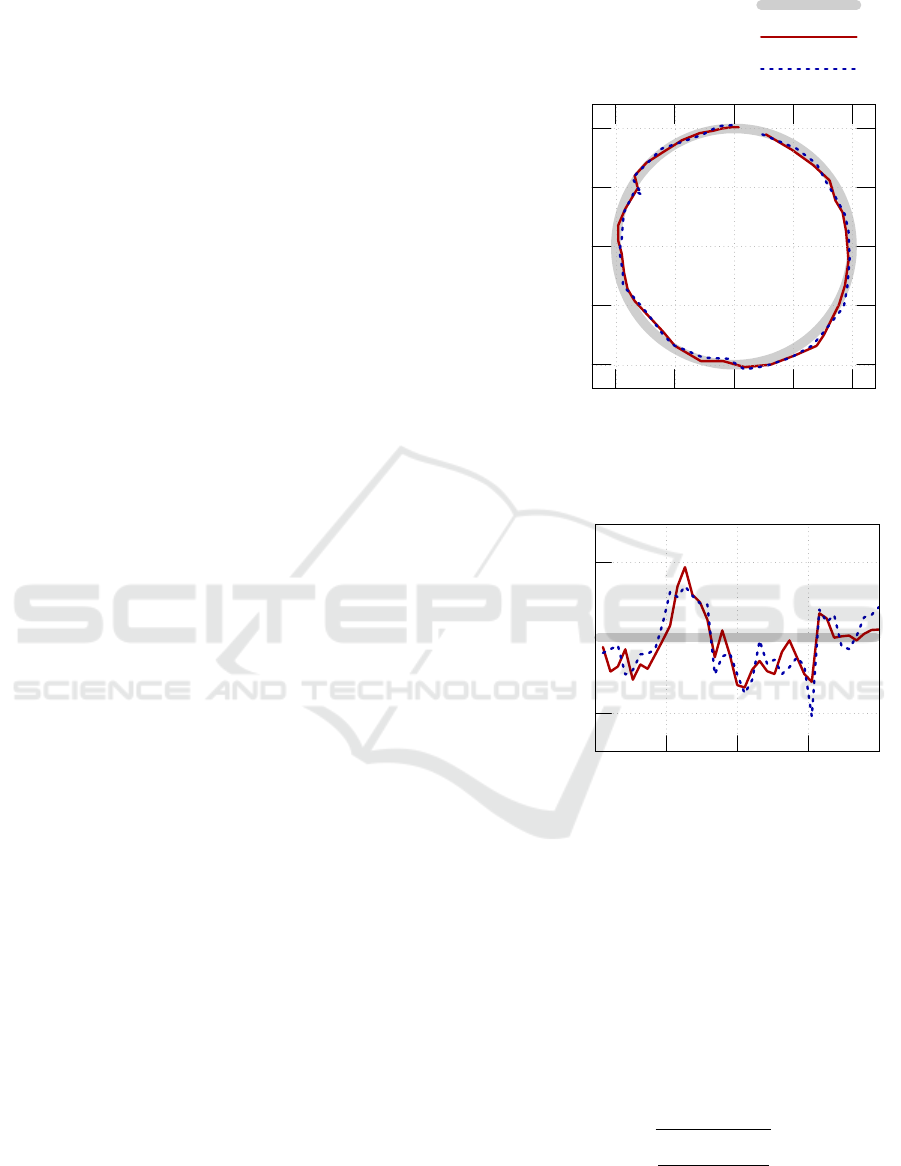
during manual mode in Fig. 5.

We use the Root-Mean-Square Deviation to com-

pute the accumulated differences in the x-y-plane (ex-

y [m]

x [m]

Target Trajectory

Onboard Sensors

External Tracking

−1

−0.5

0.5

−1 −0.5 0 0.5 1

(a) The recording in the real world state space.

0.9

1.1

0 π/2 π 3π/2

Radius [m]

Phase [rad]

(b) Transforming the trajectory to polar coordinates shows

the deviations between external tracking and onboard

sensors in more detail.

Figure 5: The shown trajectory was recorded during one of

the ten ﬂights of trajectory 6) in manual mode as depicted

in Fig. 4: A circle with diameter 2 m (depicted in grey), the

quadrocopter always pointing into the same direction. The

red line shows results from the EKF, which combines VO

and IMU data. Blue dots visualize the trajectory as recorded

by the external tracking system.

cept for experiment 2, where the z and the radial com-

ponent were used) as deﬁned:

RMSD =

∑

t=1

(

ˆs

−

)

. (4)

All results are shown in Table 2 with a graphical repre-

sentation given in Fig. 6.

VISAPP 2018 - International Conference on Computer Vision Theory and Applications

504

Table 1: Frame rates of visual odometry algorithm at different resolutions for the spherical and hyperbola mirror setup. At small

resolutions only few features are found, meaning that there is only a small difference in the transformations. As more features

are found at higher resolutions, the explicit transformation of the hyperbola mirror is about

faster (at

320 ×320px

). We

compare against the SVO algorithms results as shown in (Forster et al., 2014). However, a more powerful hardware platform

containing a quadcore processor with 1.6 GHz was used.

Mirror

160 ×160 px 320 ×320px 640 ×640 px

[Hz] [Hz] [Hz]

Spherical 29.8 ±0.1 24.4 ±0.1 15.8 ±0.1

Hyperbola 29.7 ±0.1 26.6 ±0.1 17.3 ±0.1

SVO 55 ±1 (752 ×480px)

Table 2: For each of the six trajectories (as shown in Fig. 4)

ten trials were performed. The averaged Root-Mean-Square

Deviation in the x-y-plane for these trials is shown here. In

“manual mode” the quadrocopter was moved manually on

the trajectories to eliminate problems from ﬂight control

algorithms. In “Flight Mode” trials were performed in full

ﬂight mode.

Scene

Manual Mode Flight Mode

[m] [m]

1) 0.03 ±0.01 0.07 ±0.03

2) 0.06 ±0.03 0.06 ±0.03

3) 0.07 ±0.04 0.08 ±0.04

4) 0.05 ±0.02 0.09 ±0.04

5) 0.06 ±0.03 0.11 ±0.05

6) 0.04 ±0.02 0.10 ±0.04

Average 0.05 ±0.03 0.09 ±0.04

4 DISCUSSION AND

CONCLUSION

In this paper, we have investigated a novel lightweight

omnidirectional camera setup for ﬂying robots and

tested it on a quadrocopter. The visual odometry is

combined with IMU data and the resulting pose infor-

mation is conﬁrmed using an external tracking camera.

The achieved frame rate of

26.6 ±0.1Hz

, as shown

in Table 1, is sufﬁcient for real-time application in

autonomous agents with low-power hardware. Furt-

hermore, the deviation between external tracking and

internal believe state was found to be

5 ±3 cm

in ma-

nual mode on average; in real ﬂight self localization

performs at

9 ±4cm

. The deviation was determined

in the horizontal plane for experiments 1 and 3-6 and

using the z and radial coordinates for experiment 2.

The utilized external tracking system performs already

with an error of at least

±1cm

(Haggag et al., 2013)

and thus introducing signiﬁcant uncertainty. Enhance

tracking quality currently remains future work.

While the AAV’s accuracy will be subject to furt-

0.04

0.08

0.12

0.16

1. 2. 3. 4. 5. 6. AVG

RMSD [m]

Manual Mode

Flight Mode

Figure 6: We compute the Root-Mean-Square Deviation in

the x-y-plane between external tracking and onboard sensors.

In “AVG” all six trajectories are averaged. Full results are

shown in Table 2. For each scenario 10 trials were performed

and values averaged.

her improvement, it is below the trajectory error of

the ﬂight controller and can therefore be used as a

feedback error signal to increase trajectory control pre-

cision. Thus, we have achieved our goal to enable

autonomous ﬂight in indoor or outdoor GPS-denied

areas with visual odometry.

Lastly, we will look at a real world example to

give an understanding of the error margins. For this,

we will assume a self localization error of

0.1m

and

a frame rate of

25Hz

. Furthermore, we will assume

that the AAV needs 5 frames to detect an obstacle

and initiate counter measures. Using the given frame

rate of

25Hz

, the quadrocopter needs

0.2s

to detect an

obstacle. Within these

0.2s

the safety error margin of

0.1m

(the above localization error) must not be met.

Thus, we can survey in indoor environments with a

velocity of approximately

1.8km/h

. This allows for a

broad range of application, e.g. fast search and rescue

in impassable terrain.

Our work enables autonomous robots to localize

themselves, while allowing at the same time to build

a depth map. This map offers for example obstacle

avoidance or mapping capabilities. All computations

Omnidirectional Visual Odometry for Flying Robots using Low-power Hardware

505

are performed online on embedded hardware, meaning

that the robot is able to work in unknown environments.

It can support autonomously, for example, in search

and rescue mission, disaster relief work, or exploration

tasks.

REFERENCES

Anai, T., Sasaki, T., Osaragi, K., Yamada, M., Otomo, F.,

and Otani, H. (2012). Automatic exterior orientation

procedure for low-cost uav photogrammetry using vi-

deo image tracking technique and gps information. Int.

Arch. Photogramm. Remote Sens. Spat. Inf. Sci.

Astr

om, K. J. and H

agglund, T. (2006). Advanced PID

control. ISA-The Instrumentation, Systems and Auto-

mation Society.

Augugliaro, F., Lupashin, S., Hamer, M., Male, C., Hehn, M.,

Mueller, M. W., Willmann, J. S., Gramazio, F., Kohler,

M., and D’Andrea, R. (2014). The ﬂight assembled

architecture installation: Cooperative construction with

ﬂying machines. IEEE Control Systems, 34(4):46–64.

Bay, H., Tuytelaars, T., and Van Gool, L. (2006). Surf:

Speeded up robust features. In European conference

on computer vision, pages 404–417. Springer.

Demonceaux, C., Vasseur, P., and Pegard, C. (2006). Om-

nidirectional vision on uav for attitude computation.

In IEEE International Conference on Robotics and

Automation (ICRA), pages 2842–2847.

Eberli, D., Scaramuzza, D., Weiss, S., and Siegwart, R.

(2011). Vision based position control for mavs using

one single circular landmark. Journal of Intelligent &

Robotic Systems, 61(1–4):495–512.

El-gayar, M., Soliman, H., and Meky, N. (2013). A com-

parative study of image low level feature extraction

algorithms. Egyptian Informatics Journal, 14(2):175–

181.

Engel, J., Sturm, J., and Cremers, D. (2014). Scale-aware

navigation of a low-cost quadrocopter with a monocu-

lar camera. Robotics and Autonomous Systems (RAS),

62(11):1646–1656.

Forster, C., Pizzoli, M., and Scaramuzza, D. (2014). Svo:

Fast semi-direct monocular visual odometry. In IEEE

International Conference on Robotics and Automation

(ICRA), pages 15–22.

Gaspar, J., Grossmann, E., and Santos-Victor, J. (2001). Inte-

ractive reconstruction from an omnidirectional image.

In 9th International Symposium on Intelligent Robotic

Systems (SIRS01). Citeseer.

Haggag, H., Hossny, M., Filippidis, D., Creighton, D., Na-

havandi, S., and Puri, V. (2013). Measuring depth

accuracy in rgbd cameras. In 7th International Confe-

rence on Signal Processing and Communication Sys-

tems (ICSPCS), pages 1–7.

Heinly, J., Dunn, E., and Frahm, J.-M. (2012). Compara-

tive evaluation of binary features. In Fitzgibbon, A.,

Lazebnik, S., Perona, P., Sato, Y., and Schmid, C., edi-

tors, 12th European Conference on Computer Vision

(ECCV), pages 759–773, Berlin. Springer.

Kalman, R. E. (1960). A new approach to linear ﬁltering

and prediction problems. Journal of basic Engineering,

82(1):35–45.

Lange, S., S

underhauf, N., Neubert, P., Drews, S., and Prot-

zel, P. (2012). Autonomous corridor ﬂight of a uav

using a low-cost and light-weight rgb-d camera. In

uckert, U., Joaquin, S., and Felix, W., editors, Ad-

vances in Autonomous Mini Robots: Proceedings of

the 6-th AMiRE Symposium, pages 183–192, Berlin.

Springer.

Lowe, D. G. (1999). Object recognition from local scale-

invariant features. In The proceedings of the seventh

IEEE international conference on Computer vision,

volume 2, pages 1150–1157. IEEE.

Mori, T. and Scherer, S. (2013). First results in detecting and

avoiding frontal obstacles from a monocular camera for

micro unmanned aerial vehicles. In IEEE International

Conference on Robotics and Automation (ICRA), pages

1750–1757.

Olivares-M

endez, M. A., Mondrag

on, I. F., Campoy, P., and

Mart

ınez, C. (2010). Fuzzy controller for uav-landing

task using 3d-position visual estimation. In Fuzzy

Systems (FUZZ), 2010 IEEE International Conference

on, pages 1–8.

Quigley, M., Conley, K., Gerkey, B. P., Faust, J., Foote, T.,

Leibs, J., Wheeler, R., and Ng, A. Y. (2009). Ros: an

open-source robot operating system. In ICRA Works-

hop on Open Source Software.

Remes, B., Hensen, D., Van Tienen, F., De Wagter, C.,

Van der Horst, E., and De Croon, G. (2013). Paparazzi:

how to make a swarm of parrot ar drones ﬂy autono-

mously based on gps. In IMAV 2013: Proceedings of

the International Micro Air Vehicle Conference and

Flight Competition, Toulouse, France, 17-20 Septem-

ber 2013.

Rodr

ıguez-Canosa, G. R., Thomas, S., del Cerro, J., Bar-

rientos, A., and MacDonald, B. (2012). A real-time

method to detect and track moving objects (datmo)

from unmanned aerial vehicles (uavs) using a single

camera. Remote Sensing, 4(4):1090–1111.

Rosten, E. and Drummond, T. (2006). Machine learning for

high-speed corner detection. In Leonardis, A., Bischof,

H., and Pinz, A., editors, 9th European Conference

on Computer Vision (ECCV), pages 430–443, Berlin,

Heidelberg. Springer Berlin Heidelberg.

Rublee, E., Rabaud, V., Konolige, K., and Bradski, G. (2011).

Orb: An efﬁcient alternative to sift or surf. In Internati-

onal conference on computer vision, pages 2564–2571.

IEEE.

Sch

ollig, A., Augugliaro, F., and D’Andrea, R. (2012). A

platform for dance performances with multiple quadro-

copters. Improving Tracking Performance by Learning

from Past Data, page 147.

Shi, J. and Tomasi, C. (1994). Good features to track. In

IEEE Computer Society Conference on Computer Vi-

sion and Pattern Recognition, pages 593–600. IEEE.

Teuli

ere, C., Eck, L., Marchand, E., and Gu

enard, N. (2010).

3d model-based tracking for uav position control. In

IEEE/RSJ International Conference on Intelligent Ro-

bots and Systems (IROS), pages 1084–1089.

VISAPP 2018 - International Conference on Computer Vision Theory and Applications

506

Thrun, S., Montemerlo, M., Dahlkamp, H., Stavens, D.,

Aron, A., Diebel, J., Fong, P., Gale, J., Halpenny, M.,

Hoffmann, G., Lau, K., Oakley, C., Palatucci, M., Pratt,

V., Stang, P., Strohband, S., Dupont, C., Jendrossek, L.-

E., Koelen, C., Markey, C., Rummel, C., van Niekerk,

J., Jensen, E., Alessandrini, P., Bradski, G., Davies, B.,

Ettinger, S., Kaehler, A., Neﬁan, A., and Mahoney, P.

(2006). Stanley: The robot that won the DARPA grand

challenge. Journal of Field Robotics, 23(9):661–692.

Williams, B., Cummins, M., Neira, J., Newman, P., Reid,

I., and Tard

os, J. (2009). A comparison of loop clo-

sing techniques in monocular SLAM. Robotics and

Autonomous Systems, 57(12):1188–1197. Inside Data

Association.

Omnidirectional Visual Odometry for Flying Robots using Low-power Hardware

507