
Efficient Approaches for Solving the Large-Scale k-medoids Problem
Alessio Martino, Antonello Rizzi and Fabio Massimo Frattale Mascioli
Department of Information Engineering, Electronics and Telecommunications, University of Rome ”La Sapienza”,
Via Eudossiana 18, 00184 Rome, Italy
Keywords:
Cluster Analysis, Parallel and Distributed Computing, Large-Scale Pattern Recognition, Unsupervised
Learning, Big Data Mining.
Abstract:
In this paper, we propose a novel implementation for solving the large-scale k-medoids clustering prob-
lem. Conversely to the most famous k-means, k-medoids suffers from a computationally intensive phase for
medoids evaluation, whose complexity is quadratic in space and time; thus solving this task for large datasets
and, specifically, for large clusters might be unfeasible. In order to overcome this problem, we propose two
alternatives for medoids update, one exact method and one approximate method: the former based on solving,
in a distributed fashion, the quadratic medoid update problem; the latter based on a scan and replacement
procedure. We implemented and tested our approach using the Apache Spark framework for parallel and dis-
tributed processing on several datasets of increasing dimensions, both in terms of patterns and dimensionality,
and computational results show that both approaches are efficient and effective, able to converge to the same
solutions provided by state-of-the-art k-medoids implementations and, at the same time, able to scale very
well as the dataset size and/or number of working units increase.
1 INTRODUCTION
The recent explosion of interest for Data Mining and
Knowledge Discovery put cluster analysis on the spot
again. Cluster analysis is the very basic approach in
order to extract regularities from datasets. In plain
terms, clustering a dataset consists in discovering
clusters (groups) of patterns such that similar patterns
will fall within the same cluster whereas dissimilar
patterns will fall in different clusters.
Indeed, not only different algorithms, but different
families of algorithms have been proposed in literat-
ure: partitional clustering (e.g. k-means (MacQueen,
1967; Lloyd, 1982), k-medians (Bradley et al., 1996),
k-medoids (Kaufman and Rousseeuw, 1987)), which
break the dataset into k non-overlapping clusters;
density-based clustering (e.g. DBSCAN (Ester et al.,
1996), OPTICS (Ankerst et al., 1999)) which detect
clusters as the most dense regions of the dataset; hier-
archical clustering (e.g. BIRCH (Zhang et al., 1996),
CURE (Guha et al., 1998)) where clusters are found
by (intrinsically) building a dendrogram in either a
top-down or bottom-up approach.
Moreover, in the Big Data era, the need for
clustering massive datasets emerged. Efficient and
rather easy-to-use large-scale processing frameworks
such as MapReduce (Dean and Ghemawat, 2008) or
Apache Spark (Zaharia et al., 2010) have been pro-
posed, gaining a lot of attention from Computer Sci-
ence and Machine Learning researchers alike. As
a matter of fact, several large-scale Machine Learn-
ing algorithms have been grouped in MLlib (Meng
et al., 2016), the Machine Learning library built-in in
Apache Spark.
In this work, we will focus on the k-medoids al-
gorithm, a (hard) partitional clustering algorithm sim-
ilar to the widely-known k-means. However, con-
versely to k-means, there is still some debate about a
k-medoids parallel and distributed version due to the
fact that the medoid evaluation complexity is quad-
ratic in space and time and might therefore be un-
suitable for large clusters. More into details, we
propose a novel k-medoids implementation based
on Apache Spark with two different procedures for
medoids evaluation: an exact procedure and an ap-
proximate procedure. The former, albeit exact, re-
quires the entire intra-cluster distance matrix evalu-
ation which, as already introduced, might be unsuit-
able for large clusters. The latter overcomes this prob-
lem by adopting a scan-and-replace workflow, but re-
turns a (sub)optimal medoid amongst the patterns in
the cluster at hand.
The remainder of the paper is structured as fol-
lows: Section 2 will summarise the k-medoids prob-
Martino A., Rizzi A. and Frattale Mascioli F.
Efficient Approaches for Solving the Large-Scale k-medoids Problem.
DOI: 10.5220/0006515003380347
In Proceedings of the 9th International Joint Conference on Computational Intelligence (IJCCI 2017), pages 338-347
ISBN: 978-989-758-274-5
Copyright
c
2017 by SCITEPRESS – Science and Technology Publications, Lda. All rights reserved

lem; in Section 3 the proposed approaches and re-
lated implementations will be described; in Section 4
the efficiency and effectiveness of both the proposed
medoid evaluation routines will be evaluated and dis-
cussed; Section 5 will draw some conclusions.
1.1 Contribution and State of the Art
Review
As introduced in the previous section, parallel and
distributed k-means implementations not only have
been proposed in MapReduce (Zhao et al., 2009), but
it is also included in MLlib. As far as k-medoids
is concerned, to the best of our knowledge, there
are very few parallel and distributed implementations
proposed in literature. In (Yue et al., 2016) an im-
plementation based on Hadoop/MapReduce has been
proposed where, similarly to (Zhao et al., 2009),
the Map phase evaluates the point-to-medoid assign-
ment, whereas the Reduce phase re-evaluates the new
medoids. Results show how the proposed implement-
ation scales well with the dataset size, while it lacks
of considerations regarding the effectiveness. In (Ar-
belaez and Quesada, 2013) the k-medoids problem is
decomposed (space partitioning) in many local search
problems which are solved in parallel. In (Jiang and
Zhang, 2014) the k-medoids problem is again solved
using Hadoop/MapReduce with a three-phases work-
flow (Map-Combiner-Reduce). Albeit it is unclear
how the new medoids are evaluated, the Authors show
both efficiency and effectiveness. Specifically, the lat-
ter is measured on a single labelled dataset, thus cast-
ing the clustering problem (unsupervised by defini-
tion) as a post-supervised learning problem. Both
(Yue et al., 2016) and (Jiang and Zhang, 2014) start
from Partitioning Around Medoids (PAM), the most
famous algorithm for solving the k-medoids prob-
lem (Kaufman and Rousseeuw, 2009): a greedy al-
gorithm which scans all patterns in a given cluster
and, for each point, checks whether using that point
as a medoid further minimises the objective function
(§2): if true, that point becomes the new medoid.
In this work, a k-medoids implementation based
on Apache Spark will be discussed which, due to
its caching functionalities, is more efficient than
MapReduce, especially when dealing with iterative
algorithms (§3.1).Moreover, rather than using PAM,
the (large-scale) k-medoids problem will be solved
with the implementation proposed in (Park and Jun,
2009) which has a very k-means-like workflow and
therefore it is possible to rely on a very easy-to-
parallelise algorithm flowchart.
However, the medoid(s) re-evaluation/update is a
critical task since it needs to evaluate pairwise dis-
tances amongst patterns in a given cluster in order
to find the new medoid, namely the element which
minimises the sum of distances. In order to over-
come this problem, we propose two alternatives: an
exact medoid evaluation based on cartesian product
(suitable for small/medium clusters) and an approx-
imate tracking method (suitable for large clusters as
well), proposed in (Del Vescovo et al., 2014) but never
tested on large-scale scenarios.
2 THE k-MEDOIDS CLUSTERING
PROBLEM
k-medoids is a hard partitional clustering algorithm;
it aims in partitioning the dataset S = {x
1
,x
2
,...,x
N
}
into k non-overlapping groups (clusters), i.e. S =
{S
1
,...,S
k
} such that S
i
∩ S
j
=
/
0 if i 6= j and ∪
k
i=1
S
i
=
S.
In order to find the optimal partition, k-medoids tries
to minimise the following objective function, namely
the Within-Clusters Sum-of-Distances:
WCSoD =
k
∑
i=1
∑
x∈S
i
d(x, m(i))
2
(1)
where d(·, ·) is a suitable (dis)similarity measure, usu-
ally the standard Euclidean distance, and m(i) is the
medoid for cluster i. In this work, a recent implement-
ation based on the Voronoi iteration is adopted and its
main steps can be summarised as follows:
1. select an initial set of k medoids
2. Expectation Step: assign each data point to closest
medoid
3. Maximisation Step: update each clusters’ medoid
4. Loop 2–3 until either medoids stop updating (or
their update is negligible) or a maximum number
of iterations is reached
It is worth stressing that minimising the sum of
squares (1) is an NP-hard problem (Aloise et al.,
2009) and therefore all methods (heuristics) proposed
in literature (both in terms of efficiency and effect-
iveness) strictly depend on the initial medoids: this
leaded to the implementation of initialisation heur-
istics such as k-means++ (Arthur and Vassilvitskii,
2007) or DBCRIMES (Bianchi et al., 2016).
It has already been discussed that evaluating the
medoid is more complex than evaluating the mean,
since it requires the complete pairwise distance mat-
rix D between all points in a given cluster S
h
, form-
ally defined as an |S
h
|×|S
h
| real-valued matrix whose
generic entry is given by
D
(S
h
)
i, j
= d(x
i
,x
j
) (2)

or, as far as the Euclidean distance is concerned, du-
ally definable in terms of Gram matrix as
D
(S
h
)
i, j
=
q
G
(S
h
)
i, j
=
q
hx
i
− x
j
,x
i
− x
j
i (3)
for any two patterns x
i
, x
j
∈ S
h
.
Despite its complexity, by minimising the sum of
pairwise distances rather than the squared Euclidean
distance from the average point (i.e. k-means), k-
medoids is more robust with respect to noise and out-
liers. Moreover, k-medoids is particularly suited if the
cluster prototype must be an element of the dataset
(the same is generally not true for k-means) and it is
applicable to ideally any input space, not necessarily
metric, since there is no need to define an algebraic
structure in order to compute the representative ele-
ment of a cluster.
3 PROPOSED APPROACH
3.1 A Quick Spark Introduction
In this work Apache Spark (hereinafter simply Spark)
has been chosen over Hadoop/MapReduce due to its
efficiency, as introduced in §1.1. Indeed, MapRe-
duce forces any algorithm pipeline into a sequence of
Map → Reduce steps, eventually with an intermediate
Combiner phase, which strains the implementation of
more complex operations such as joins or filters as
they have to be casted as well into Map → Reduce. In
MapReduce, computing nodes do not have memory of
past executions: this does not suit the implementation
of iterative algorithms, as the master process must for-
ward data to workers at each MapReduce job, which
typically corresponds to a single iteration of a given
algorithm.
Spark overcomes these problems as it includes
highly efficient map, reduce, join, filter (and many
others) operations which are not only natively dis-
tributed, but can be arbitrarily pipelined together. As
far as iterative algorithms are concerned, Spark offers
caching in memory and/or disk, therefore there is no
need to forward data back and forth from/to workers
at each iteration.
Atomic data structures in Spark are the so-
called Resilient Distributed Datasets (RDDs): distrib-
uted (across workers
1
) collection of data with fault-
tolerance mechanisms, which can be created start-
ing from many sources (distributed file systems, data-
1
In Spark, workers are the elementary computational
units, which can be either single cores on a CPU or en-
tire computers, depending on the environment configuration
(i.e. the Spark Context).
bases, text files and the like) or by applying trans-
formations on other RDDs.
Example of transformations which will turn useful
in the following subsections are:
map(): RDD2 = RDD1.map( f )
creates RDD2 by applying function f to every ele-
ment in RDD1
f ilter(): RDD2 = RDD1. f ilter(pred)
creates RDD2 by filtering elements from RDD1
which satisfy predicate pred (i.e. if pred is True)
reduceByKey(): RDD2 = RDD1.reduceByKey( f )
creates RDD2 by merging according to function f
all values for each key in RDD1: RDD2 will have
the same keys as RDD1 and a new value obtained
by the merging function.
Similarly, examples of actions which can be applied
to RDDs are:
count(): RDD.count()
count the number of elements in RDD
collect(): RDD.collect()
collects in-memory on the master node the entire
RDD content.
3.2 Main Algorithm
The main parallel and distributed k-medoids flowchart
is summarised in the Algorithm 1.
It is possible to figure datasetRDD to be a key-value
pair RDD
2
or, in other words, an RDD where each
record has the form hkey ; valuei. Specifically, the
key is a sequential integer ID and the value is (as a
first approach) an n-dimensional real-valued vector.
At the beginning of each iteration, a new key-
value pair RDD will be created (distancesRDD)
where the key is still the pattern ID whereas, the
value (distanceVector) is a k-dimensional real-
valued vector where the i
th
element contains the dis-
tance with the i
th
medoid. The following two RDDs
(nearestDistRDD and nearestClusterRDD) map
the pattern ID with the nearest distance value and the
nearest cluster ID (i.e. medoid), respectively. These
evaluations end the Maximisation Step for the Voro-
noi iteration (§2).
nearestClusterRDD is the main RDD for the
medoids update step (i.e. the Expectation Step
for the Voronoi iteration): after gathering the list
2
In the following subsections and pseudocodes every
variable whose name ends with RDD shall be considered as
an RDD, therefore a data structure whose shards are distrib-
uted across the workers or, similarly, with no guarantee that
a single worker has its entire content in memory.

of pattern IDs (patternsInClusterIDs) belong-
ing to cluster ID clID, an additional RDD contain-
ing the patterns belonging to clID will be created
(patternsInClusterRDD). This RDD, which still is
a key-value pair RDD, is the main input for the
medoids update step which we shall discuss in more
details in the following subsection.
1 Begin main
2 Load datasetRDD from source (e.g. text-
file);
3 Cache datasetRDD on workers;
4 Set maxIterations, k,
approximateTrackingFlag;
5 medoids = initialSeeds();
6 for iter in range(1:maxIterations)
7 previousMedoids = medoids;
8 distancesRDD = datasetRDD.map(d(
pattern,medoids));
9 nearestDistRDD = distancesRDD.map(min(
distanceVector));
10 nearestClusterRDD = distancesRDD.map(
argmin(distanceVector));
11 for clID in range(1:k)
12 patternsInClusterIDs =
nearestClusterRDD.filter(clusterID
== clID);
13 patternsInClusterRDD =
nearestClusterRDD.filter(clusterID
in patternsInClusterIDs);
14 if approximateTrackinFlag is True
15 medoids[clID] =
approximateMedoidTracking();
16 else
17 medoids[clID] =
exactMedoidUpdate();
18 WCSoD = nearestDistRDD.values().sum();
19 if stopping criteria == True
20 break;
21 End main
Algorithm 1: Pseudocode for the main k-medoids skeleton
(namely, Voronoi iterations).
3.3 Updating Medoids
3.3.1 Exact Medoid Update
The Exact Medoid Update consists in evaluating the
pairwise distance matrix amongst all the patterns in a
given cluster and then finding the element which min-
imises the sum by rows/columns
3
of such matrix.
We define a-priori a parameter T , a threshold value
3
In the following, we suppose that the (dis)similarity
measure d(·,·) is metric, therefore satisfies the symmetry
property, i.e. d(a,b) = d(b,a). For metric (dis)similarity
measures the pairwise distance matrix is symmetric by
definition and the sum by rows or columns leads to the same
result.
which states the maximum allowed cluster cardinal-
ity in order to consider such cluster as ”small”. This
parameter can be tuned considering both the expected
clusters’ sizes and the amount of memory available on
the master node.
1 Begin function exactMedoidUpdate(
patternsInClusterRDD)
2 if patternsInClusterRDD.count() < T
3 patterns = patternsInClusterRDD.
collect().asmatrix();
4 distanceMatrix = pdist(patterns,d);
5 Sum distanceMatrix by rows or columns;
6 medoidID = argmin of rows/columns sum;
7 return patterns[medoidID];
8 else
9 pairsRDD = patternsInClusterRDD.
cartesian(patternsInClusterRDD);
10 distancesRDD = pairsRDD.map(d(pattern1
,pattern2));
11 distancesRDD = distancesRDD.
reduceByKey(add);
12 medoidID = distancesRDD.min(key=dist);
13 return patternsInClusterRDD.filter(ID
== medoidID).collect();
14 End function
Algorithm 2: Pseudocode for the Exact Medoid Update
routine.
Algorithm 2 describes the Exact Medoid Update
routine. Basically, if the cluster is ”small” it is pos-
sible to collect on the master node the entire set of pat-
terns and therefore use one of the many in-memory al-
gorithms (pdist) for evaluating the pairwise distance
matrix according to a given (dis)similarity measure d.
Conversely, if the cluster is ”not-small”, via Spark
it is possible to evaluate the cartesian product of
this cluster’s RDD with itself, leading to a new
RDD (pairsRDD) where each record is a pair of re-
cords from the original RDD, therefore it is pos-
sible to figure pairsRDD to have the form hID1 ;
pattern1 ; ID2 ; pattern2i. Given these pairs, eval-
uating the (dis)similarity measure is straightforward
and distancesRDD will have the form hID1 ; ID2
; d(pattern1,pattern2)i. Given the analogy with the
pairwise distance matrix, in order to perform the sum
by rows or columns, distancesRDD will be reduced
by using either the ID of the first pattern (by rows) or
the ID of the second pattern (by columns) as key and
using the addition operator to values. In other words,
for ID1 (or ID2) we sum all the distances with other
IDs (i.e. other patterns). Given these sums, the final
step consists in evaluating the minimum of the result-
ing RDD considering the sum of distances rather than
the ID leading to medoidID, the ID of the new medoid
which will be filtered from patternsInClusterRDD
and returned as the new, updated, medoid.

3.3.2 Approximate Medoid Tracking
Whilst the (large scale) Exact Medoid Update (Al-
gorithm 2, namely the else branch) relies on natively
distributed and highly efficient Spark operations,
the cartesian product might be unfeasible for very
large clusters since it creates an RDD whose size is
squared the size of the cluster (i.e. squared the size of
the input RDD) according to Eqs. (2)-(3).
1 Begin function approximateMedoidTracking(
patternsInClusterRDD,medoids,clusterID)
2 if patternsInClusterRDD.count() < P
3 patterns = patternsInClusterRDD.
collect().asmatrix();
4 distanceMatrix = pdist(patterns,d);
5 Sum distanceMatrix by rows or columns;
6 medoidID = argmin of rows/columns sum;
7 return patterns[medoidID];
8 else
9 pool = patternsInClusterRDD.filter(ID
in range(1:P)).collect().asmatrix();
10 patternsInClusterRDD =
patternsInClusterRDD.filter(ID not in
range(1:P));
11 for pattern in patternsInClusterRDD
12 Extract x1!=x2 from pool;
13 if d(x1,medoids[clusterID])>=d(x2,
medoids[clusterID])
14 Remove x1 from pool;
15 else
16 Remove x2 from pool;
17 pool = pool.append(pattern);
18 distanceMatrix = pdist(pool,d);
19 Sum distanceMatrix by rows or columns;
20 medoidID = argmin of rows/columns sum;
21 return pool[medoidID];
22 End function
Algorithm 3: Pseudocode for the Approximate Medoid
Tracking routine.
To this end, a second, approximate, medoid evalu-
ation based on (Del Vescovo et al., 2014) is proposed.
For the sake of ease, their findings can be summarised
as follows:
1. set a pool size P and fill the pool with the first P
patterns from the cluster at hand
2. for every remaining pattern x, select uniformly at
random two items from the pool (x
1
and x
2
) and
check their distances with the current medoid m.
If d(x
1
,m) ≥ d(x
2
,m), remove x
1
from the pool;
otherwise remove x
2
. Finally, insert x in the pool.
3. evaluate the new medoid with any standard in-
memory routine using the patterns in the pool.
Algorithm 3 describes the Approximate Medoid
Tracking routine. As in Algorithm 2, if the cluster
is ”small” there is not need to trigger any parallel an-
d/or distributed medoid evaluation which can thus be
done locally, in an exact manner. Conversely, if the
cluster is ”not-small” the first P items will be cached
and removed from the RDD which contains the pat-
terns in such cluster. Finally, the approximate proced-
ure starts by iterating over the RDD and performing
the steps from (Del Vescovo et al., 2014).
3.4 Selecting Initial Seeds
As discussed in §2, the solution returned by heurist-
ics such as k-medoids is strictly dependent from the
initial medoids (seeds) selection. One of the most
widely-used approaches consists in random selection
and multi-start: a given number (typically 5 or 10)
of sets of k initial medoids are uniformly at random
selected from the dataset and for each set of initial
medoids the k-medoids algorithm will be run. The fi-
nal clustering solution is determined by the run with
minimum WCSoD. Other solutions have been pro-
posed in literature such as k-means++ which we im-
plemented for a more accurate seeds selection. In its
standard form, k-means++ works as follows:
1. select the first centroid
4
uniformly at random from
the dataset S
2. evaluate pairwise distances between patterns and
already-selected centroid, mapping each pattern
with its closest centroid; let us call D(x) the
closest distance between pattern x ∈ S and the
already-selected centroids
3. a pattern from the dataset S is selected as new
centroid with probability
D
2
(x)
∑
x∈S
D
2
(x)
4. Loop 2–3 until k initial centroids are selected
The Spark k-means++ distributed version is summar-
ised in Algorithm 4.
Many of these RDDs have already been introduced
in §3.2 and, since step #2 in k-means++ actually is
the Maximisation step for the Voronoi iteration (§2),
such RDDs will be created and evaluated in the same
manner as described in Algorithm 1. One might ob-
ject that collecting (i.e. loading into the master node
memory) nearestDistRDD might not be suitable for
large datasets. It is worth noticing that, in order to
save space, only the distance values and not the IDs
will be collected and, moreover, a modern computer
can store several millions of elements within an in-
memory array. Therefore (as a first approach) we do
4
Historically, k-means++ was designed for k-means and
therefore we will refer to the cluster representative as
”centroid”. However, since it returns k data points as ini-
tial seeds, the same procedure holds for ”medoid”.

not consider this operation as prohibitive.
1 Begin function initialSeeds(datasetRDD,k)
2 N = datasetRDD.count();
3 firstMedoidID = random.integer(1,N);
4 medoids = datasetRDD.filter(ID ==
firstMedoidID);
5 for iter in range(1:k-1)
6 distancesRDD = datasetRDD.map(d(
pattern,medoids));
7 nearestDistRDD = distancesRDD.map(min(
distanceVector));
8 distances = nearestDistRDD.values().
collect();
9 distances = distances/sum(distances);
10 newMedoidID = random.choice(range(1:N)
,prob=distances);
11 medoids = medoids.append(datasetRDD.
filter(ID == newMedoidID).collect());
12 End function
Algorithm 4: Pseudocode for k-means++.
4 COMPUTATIONAL RESULTS
4.1 Datasets and Environment
Description
In order to show both the effectiveness and the ef-
ficiency of the proposed algorithm, 9 datasets have
been considered. All of them are freely available
from UCI Machine Learning Repository (Lichman,
2013) and their major characteristics are summarised
in Table 1. Classes in labelled datasets (e.g. Wine,
Iris) and eventual pattern IDs (e.g. 3D Road Network)
have been deliberately discarded. All datasets have
been normalised before processing.
Table 1: List of datasets used for analysis.
Dataset Name # patterns # features
US Census 1990 2458285 68
3D Road Network 434874 4
KEGG Metabolic Relation
Network (Directed)
53413 23
Bag of Words (ENRON) 39861 28102
Daily and Sport Activities 9120 5625
Bag of Words (KOS) 3430 6906
Bag of Words (NIPS) 1500 12419
Iris 178 13
Wine 150 4
Experiments shown in §4.2 and 4.3 have been con-
ducted on a Linux Ubuntu 16.04LTS workstation with
two Intel
R
Xeon
R
CPUs @2.60GHz for a total of 24
physical cores, 32GB RAM and 1TB HDD. Such 24
cores have been grouped in 6 groups of 4 cores each,
in order to simulate 6 PCs working in parallel which
will be the workers for these experiments. The latest
Apache Spark version has been used (v2.2.0) and,
specifically, its Python API (namely, PySpark) driven
by Python v2.7.13 with NumPy v1.12.1 (van der Walt
et al., 2011) for efficient numerical computations.
4.2 Effectiveness
In order to show the effectiveness of the proposed
distributed implementation, the clustering problem
has not been casted as a semi-supervised or post-
supervised learning problem since, in our opinion,
this is not a good way to address the effectiveness
of a clustering algorithm (which solves unsupervised
problems by definition) as one might tend to con-
fuse clusters with classes. Rather, the solution (i.e.
the objective function) returned by the distributed k-
medoids implementation will be compared with the
solution returned by a well-established and not dis-
tributed k-medoids implementation, specifically the
one available in the MATLAB
R
R2015a.
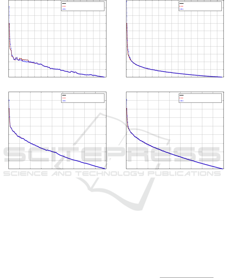
In Figure 1 the objective function returned by
the distributed implementation is shown, considering
both the Approximate Medoid Tracking and the Exact
Medoid Update routines for medoids update, against
the MATLAB k-medoids implementation. We con-
sidered the two smaller datasets (Iris and Wine in Fig-
ures 1(a) and 1(b), respectively) in order to be able
to test every possible value for k; that is, from 1 up
to the singleton (i.e. the total number of patterns).
To ensure a fair comparison, the same (dis)similarity
measure has been used (standard Euclidean distance)
but, more importantly, the three competitors started
from the very same initial seeds
5
. Since the Approx-
imate Medoid Tracking has some randomness (i.e. its
replacement policy), for every k the average objective
function value across 5 runs is shown.
Clearly, Figure 1 shows that the proposed ap-
proach is effective. Specifically, when using the Ex-
act Medoid Update, it returns the very same objective
function value
6
when compared to the state-of-the-art
(albeit local) MATLAB implementation. The Approx-
imate Medoid Tracking has surprising results as well,
especially for Wine (Figure 1(b)).
Similarly, in Figures 2(a) and 2(b) the results
when using k-means++ rather than manual (i.e. de-
terministic) selection for initial medoids is shown. As
in the previous case, the two figures regard Iris and
Wine datasets, respectively.
5
Specifically, for k = i the first i patterns have been se-
lected as initial seeds.
6
Therefore returns the very same medoids and the very
same point-to-medoid assignments.
0 10 20 30 40
50 60
70 80 90 100 110 120 130 140
150
0
10
20
30
40
50
60
70
80
90
100
k
WCSoD
Spark w/ Exact Medoid Update
Matlab
Spark w/ Approximate Medoid Tracking
(a) Iris Dataset
0 20 40
60
80 100 120 140
160
180
0
20
40
60
80
100
120
140
160
180
k
WCSoD
Spark w/ Exact Medoid Update
Matlab
Spark w/ Approximate Medoid Tracking
(b) Wine Dataset
Figure 1: Effectiveness tests with deterministic initial seeds
selection.
Figure 2 does not only confirm that the distrib-
uted k-medoids implementation is effective, but also
that the distributed k-means++ implementation works
very well. Obviously, since k-means++ has random
behaviour, 5 runs have been performed for each com-
petitor and the average objective function is shown.
Finally, it is worth stressing that a threshold of
T = 20 patterns for both datasets has been used.
Certainly the pool size for the Approximate Medoid
Tracking has a major impact on the tracking quality
itself: since the pool must fit in memory (as we ex-
pect from a ”small cluster”), we dually used T ≡ P
to indicate the pool size as well. For the sake of ease
and shorthand we omit any tests regarding how the
medoid tracking quality and the procedure complex-
ity changes as a function of the pool size: such results
have been discussed in (Del Vescovo et al., 2014), to
which we refer the interested reader.
0 10 20 30 40
50 60
70 80 90 100 110 120 130 140
150
0
10
20
30
40
50
60
70
80
90
100
k
WCSoD
Spark w/ Exact Medoid Update
Matlab
Spark w/ Approximate Medoid Tracking
(a) Iris Dataset
0 20 40
60
80 100 120 140
160
180
0
20
40
60
80
100
120
140
160
180
k
WCSoD
Spark w/ Exact Medoid Update
Matlab
Spark w/ Approximate Medoid Tracking
(b) Wine Dataset
Figure 2: Effectiveness tests with k-means++ initial seeds
selection.
4.3 Efficiency
In order to address the efficiency of the proposed im-
plementation, the aim of this subsection is to show
whether it respects the speedup and sizeup properties,
defined as follows (Xu et al., 1999):
speedup measures the ability of the parallel and dis-
tributed algorithm to reduce the running time as
more workers are considered. More formally, the
dataset size is kept constant and the number of
workers will increase from 1 to m. The speedup
for an m-nodes cluster is defined as:
speedup(m) =
running time on 1 worker
running time on m workers
sizeup measures the ability of the parallel and dis-
tributed algorithm to manage an m times larger
dataset while keeping the number of workers con-
stant. The speedup for an m times larger dataset is
defined as:
sizeup(S,m) =
running time for processing m × S
running time for processing S
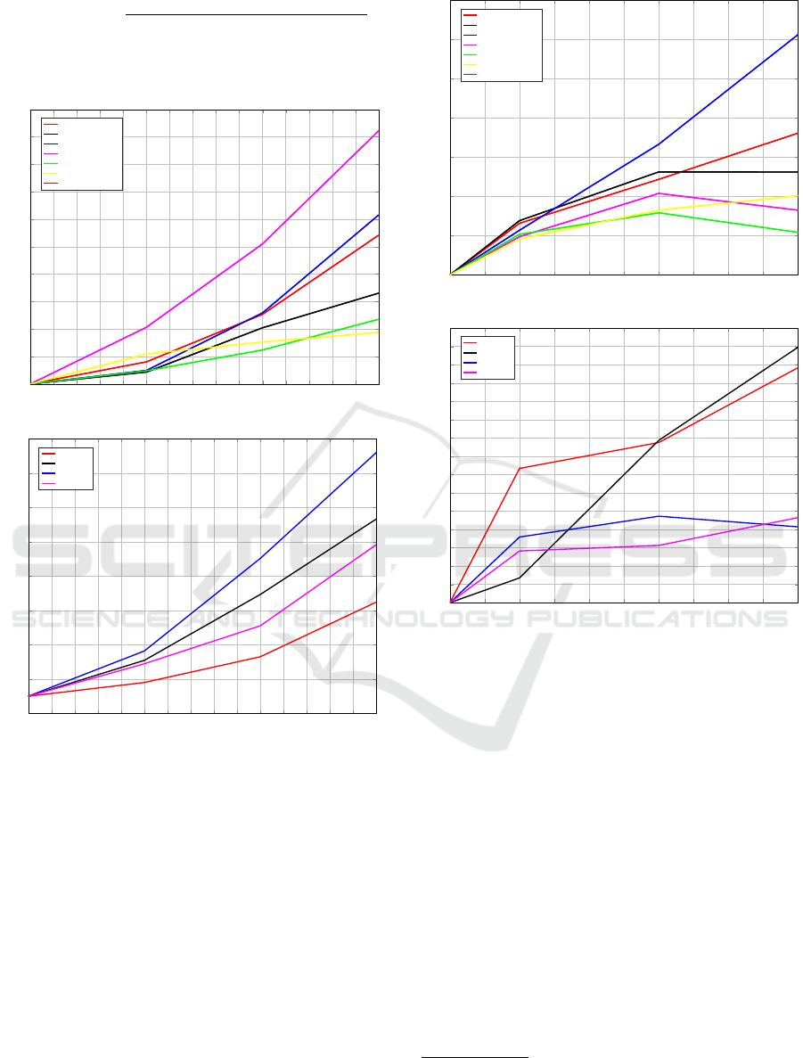
Figure 3 shows the sizeup performances for both
1 1.2 1.4
1.6
1.8 2 2.2 2.4
2.6
2.8 3 3.2 3.4
3.6
3.8 4
1
1.5
2
2.5
3
3.5
4
4.5
5
5.5
6
Dataset increasing factor m
Sizeup
Activities
KEGG
Census
3D Road Network
KOS
NIPS
ENRON
(a) Approximate Medoid Tracking
1 1.2 1.4
1.6
1.8 2 2.2 2.4
2.6
2.8 3 3.2 3.4
3.6
3.8 4
0
2
4
6
8
10
12
14
16
Dataset increasing factor m
Sizeup
Activities
KEGG
NIPS
KOS
(b) Exact Medoid Update
Figure 3: Sizeup.
the medoid update routines. Specifically, the sizeup
parameter m has been set to m = 1,2,3,4. All of
the workers available and all but Wine and Iris data-
sets from Table 1 have been used. Figure 3(a) de-
picts the Approximate Medoid Tracking case which
has a very good sizeup performances, especially for
m ≥ 3 (e.g. a 4-times larger dataset needs from 1.9
to 5.5 times more time). Figure 3(b) depicts the Ex-
act Medoid Update case which has generally lower
performances with respect to the former. However,
as the dataset size increases, the performances tend
to improve (e.g. for KEGG a 4-times larger problem
needs 11-times more time, whereas for Activities it
needs 6-times more time) but, on the other hand, this
approach cannot be adopted for larger datasets under
1
1.5
2
2.5
3
3.5
4
4.5 5 5.5 6
1
1.5
2
2.5
3
3.5
4
4.5
# of workers
Speedup
Activities
KEGG
Census
3D Road Network
KOS
NIPS
ENRON
(a) Approximate Medoid Tracking
1
1.5
2
2.5
3
3.5
4
4.5 5 5.5 6
1
1.2
1.4
1.6
1.8
2
2.2
2.4
2.6
2.8
3
3.2
3.4
3.6
3.8
4
# of workers
Speedup
Activities
KEGG
NIPS
KOS
(b) Exact Medoid Update
Figure 4: Speedup.
reasonable running times
7
.
For the speedup, 1, 2, 4 and 6 workers and the
same datasets as for the sizeup experiment have been
used.
The algorithm has very good speedup perform-
ances when using the Approximate Medoid Update,
Figure 4(a): the bigger the dataset, the better the spee-
dup. For some datasets (typically the smallest ones)
implying more than 4 workers does not improve the
overall performances; indeed, since they are rather
small and due to the Approximate Medoid Track-
ing routine being computationally lighter (§4.4), a
massive parallelisation will unlikely be helpful as
most of the time will be spent in scheduling/commu-
nication tasks rather than pure processing.
Figure 4(b), finally, shows the Exact Medoid Up-
date case, which has very good speedup performances
7
Whilst using all of the workers available, updating the
medoid for a 100000-patterns cluster took more than 3
hours.

as well. Indeed, due to the intensive parallel evalu-
ations required for solving the exact evaluation, more
workers are crucial for speeding-up such phase. The
above reasoning regarding smaller datasets still holds.
For the sake of completeness and comparison, in
Table 2 the absolute running times for the Activities
dataset have been reported.
Table 2: Absolute running times in minutes.
# workers Approximate Exact
1 2 30
2 1.3 13
4 0.97 11
6 0.76 8.5
4.4 On Computational Complexity
An additional reason for choosing the implementation
proposed in (Park and Jun, 2009) over other imple-
mentations such as the most famous PAM for solv-
ing the k-medoids problem lies in its complexity. In-
deed, since the chosen implementation is based on the
Voronoi iterations as in k-means, the two algorithms
have the same complexity, that is O(nk) per-iteration,
where n is the number of data points and k is the num-
ber of clusters. For the sake of comparison, PAM has
a per-iteration complexity of O(k(n − k)
2
) (Ng and
Han, 1994), making it unsuitable for large datasets.
In this work, patterns have been considered as d-
dimensional real-valued vectors and, moreover, such
input space has been equipped with the Euclidean dis-
tance as (dis)similarity measure, whose complexity is
O(d). Therefore, the overall per-iteration complex-
ity can as well be defined as O(nkd). By considering
p computational units, the per-iteration complexity
drops to O(nk/p) (or O(nkd/p) by explicitly taking
into account the Euclidean distance) since the point-
to-medoids distance will be computed in parallel.
As far as the medoid update is concerned, the
Exact Medoid Update procedure has complexity
O(c
2
/p) where c is the cluster size, whereas the Ap-
proximate Medoid Tracking has complexity O(c −
P) ' O(c) since usually c P.
5 CONCLUSIONS
In this paper, we proposed a novel implementation for
the large-scale k-medoids algorithm using the Apache
Spark framework as parallel and distributed comput-
ing environment. Specifically, we proposed two pro-
cedures for the medoid evaluation: an exact (but com-
putationally intensive) procedure and an approximate
(but computationally lighter) procedure which have
been proved to be very effective. As far as efficiency
is concerned, we tested our algorithm in a single-
machine multi-threaded environment with satisfact-
ory results.
Starting from this implementation many further
steps can be done. First, this implementation has
been deliberately proposed to be as general as pos-
sible: indeed, by looking at the algorithm description
in §3.2, 3.3 and 3.4, the end-user must just change the
(dis)similarity measure d(·,·) according to the nature
of the input space at hand in order for the whole im-
plementation to work. The same reasoning holds for
k-means++: albeit it is true that there are efficient par-
allel and distributed implementations (e.g. k-means||,
(Bahmani et al., 2012)), they namely work on the Eu-
clidean space only. Moreover, as concerns initialisa-
tion techniques, a future work might focus on devel-
oping a DBCRIMES parallel and distributed imple-
mentation, since it is also suitable for dealing with
non-metric spaces.
Further, we proposed two medoid evaluation pro-
cedures which are ideally robust to any cluster’s size.
This can be seen in Algorithm 1, where a for-loop
scans one cluster at the time. This is robust because
the entire processing power is dedicated to a single
cluster which can therefore be massive as well, but if
one is confident that clusters cannot be arbitrarily big
it is possible to group the available workers
8
in such
way that each group processes a given cluster. In this
manner the aforementioned for-loop can be done in
parallel as well.
Albeit the two medoids’ update routines have been
presented separately in order to discuss their respect-
ive strengths and weaknesses, they can be easily used
together by adopting a double-threshold approach.
Specifically, let T
1
and T
2
be two thresholds with
T
1
< T
2
: every cluster whose size is less than T
1
can be considered as ”small” and processed fully in-
memory; every cluster whose size is in range [T
1
,T
2
]
can be considered as ”medium” and processed using
the Exact Medoid Update and, finally, clusters greater
than T
2
, to be considered as ”big”, can be processed
using the Approximate Medoid Tracking.
One of the most intriguing works is a direct
extension of the former observation, as discussed
in §2: ideally the k-medoids can work with any
(dis)similarity measure and it does not need to define
some operations for evaluating the new cluster repres-
entative (e.g. mean or median): whether it is possible
to define a (dis)similarity measure between two ob-
jects, the k-medoids can be used. This opens a new
horizon on the nature of the input space(s) which can
8
As we did in order to simulate 4-core PCs.

be clustered, as the so-called non-metric spaces such
as graphs or sequences, for which defining a mean or
median is nonsensical.
REFERENCES
Aloise, D., Deshpande, A., Hansen, P., and Popat, P. (2009).
Np-hardness of euclidean sum-of-squares clustering.
Machine learning, 75(2):245–248.
Ankerst, M., Breunig, M. M., Kriegel, H.-P., and Sander, J.
(1999). Optics: Ordering points to identify the clus-
tering structure. In Proceedings of the 1999 ACM
SIGMOD International Conference on Management
of Data, SIGMOD ’99, pages 49–60, New York, NY,
USA. ACM.
Arbelaez, A. and Quesada, L. (2013). Parallelising the k-
medoids clustering problem using space-partitioning.
In Sixth Annual Symposium on Combinatorial Search.
Arthur, D. and Vassilvitskii, S. (2007). k-means++: The
advantages of careful seeding. In Proceedings of the
eighteenth annual ACM-SIAM symposium on Discrete
algorithms, pages 1027–1035. Society for Industrial
and Applied Mathematics.
Bahmani, B., Moseley, B., Vattani, A., Kumar, R., and
Vassilvitskii, S. (2012). Scalable k-means++. Pro-
ceedings of the VLDB Endowment, 5(7):622–633.
Bianchi, F. M., Livi, L., and Rizzi, A. (2016). Two
density-based k-means initialization algorithms for
non-metric data clustering. Pattern Analysis and Ap-
plications, 3(19):745–763.
Bradley, P. S., Mangasarian, O. L., and Street, W. N. (1996).
Clustering via concave minimization. In Proceedings
of the 9th International Conference on Neural Inform-
ation Processing Systems, NIPS’96, pages 368–374,
Cambridge, MA, USA. MIT Press.
Dean, J. and Ghemawat, S. (2008). Mapreduce: simplified
data processing on large clusters. Communications of
the ACM, 51(1):107–113.
Del Vescovo, G., Livi, L., Frattale Mascioli, F. M., and
Rizzi, A. (2014). On the problem of modeling struc-
tured data with the minsod representative. Interna-
tional Journal of Computer Theory and Engineering,
6(1):9.
Ester, M., Kriegel, H.-P., Sander, J., Xu, X., et al. (1996).
A density-based algorithm for discovering clusters in
large spatial databases with noise. In Proceedings of
the Second International Conference on Knowledge
Discovery and Data Mining, volume 96, pages 226–
231.
Guha, S., Rastogi, R., and Shim, K. (1998). Cure: An ef-
ficient clustering algorithm for large databases. SIG-
MOD Rec., 27(2):73–84.
Jiang, Y. and Zhang, J. (2014). Parallel k-medoids cluster-
ing algorithm based on hadoop. In Software Engin-
eering and Service Science (ICSESS), 2014 5th IEEE
International Conference on, pages 649–652. IEEE.
Kaufman, L. and Rousseeuw, P. J. (1987). Clustering by
means of medoids. Statistical Data Analysis Based
on the L1-Norm and Related Methods, pages North–
Holland.
Kaufman, L. and Rousseeuw, P. J. (2009). Finding groups
in data: an introduction to cluster analysis, volume
344. John Wiley & Sons.
Lichman, M. (2013). UCI machine learning repository.
Lloyd, S. (1982). Least squares quantization in pcm. IEEE
transactions on information theory, 28(2):129–137.
MacQueen, J. B. (1967). Some methods for classification
and analysis of multivariate observations. In Cam, L.
M. L. and Neyman, J., editors, Proc. of the fifth Berke-
ley Symposium on Mathematical Statistics and Prob-
ability, volume 1, pages 281–297. University of Cali-
fornia Press.
Meng, X., Bradley, J., Yavuz, B., Sparks, E., Venkatara-
man, S., Liu, D., Freeman, J., Tsai, D., Amde, M.,
Owen, S., et al. (2016). Mllib: Machine learning in
apache spark. Journal of Machine Learning Research,
17(34):1–7.
Ng, R. T. and Han, J. (1994). Efficient and effective cluster-
ing methods for spatial data mining. In Proceedings
of the 20th International Conference on Very Large
Data Bases, VLDB ’94, pages 144–155, San Fran-
cisco, CA, USA. Morgan Kaufmann Publishers Inc.
Park, H.-S. and Jun, C.-H. (2009). A simple and fast al-
gorithm for k-medoids clustering. Expert systems with
applications, 36(2):3336–3341.
van der Walt, S., Colbert, S. C., and Varoquaux, G. (2011).
The numpy array: A structure for efficient numerical
computation. Computing in Science & Engineering,
13(2):22–30.
Xu, X., J
¨
ager, J., and Kriegel, H.-P. (1999). A fast parallel
clustering algorithm for large spatial databases. Data
Mining and Knowledge Discovery, 3(3):263–290.
Yue, X., Man, W., Yue, J., and Liu, G. (2016). Paral-
lel k-medoids++ spatial clustering algorithm based on
mapreduce. arXiv preprint arXiv:1608.06861.
Zaharia, M., Chowdhury, M., Franklin, M. J., Shenker, S.,
and Stoica, I. (2010). Spark: Cluster computing with
working sets. HotCloud, 10(10-10):95.
Zhang, T., Ramakrishnan, R., and Livny, M. (1996). Birch:
An efficient data clustering method for very large
databases. In Proceedings of the 1996 ACM SIGMOD
International Conference on Management of Data,
SIGMOD ’96, pages 103–114, New York, NY, USA.
ACM.
Zhao, W., Ma, H., and He, Q. (2009). Parallel k-means
clustering based on mapreduce. In IEEE Interna-
tional Conference on Cloud Computing, pages 674–
679. Springer.
