The Challenge of using Map-reduce to Query Open Data

Mauro Pelucchi

, Giuseppe Psaila

and Maurizio Toccu

University of Bergamo, Italy (current afﬁliation: Tabulaex srl, Milan, Italy)

University of Bergamo, Italy

University of Milano Bicocca, Italy

Keywords:

Retrieval of Open Data, Single Item Extraction, Map-reduce.

Abstract:

For transparency and democracy reasons, a few years ago Public Administrations started publishing data sets

concerning public services and territories. These data sets are called open, because they are publicly available

through many web sites.

Due to the rapid growth of open data corpora, both in terms of number of corpora and in terms of open data

sets available in each single corpus, the need for a centralized query engine arises, able to select single data

items from within a mess of heterogeneous open data sets. We gave a ﬁrst answer to this need in (Pelucchi

et al., 2017), where we deﬁned a technique for blindly querying a corpus of open data. In this paper, we face

the challenge of implementing this technique on top of the Map-Reduce approach, the most famous solution

to parallelize computational tasks in the Big Data world.

1 INTRODUCTION

Public Administrations, like central and local govern-

ments, are publishing more and more data sets con-

cerning their activities and citizens. Since these data

sets are open, i.e., publicly available for any interested

people and organizations, they are called Open Data.

The motivation for such an effort is transparency, a

key factor in democracy. However, in (Carrara et al.,

2015) the notion of Open Data Value Chain has been

introduced: the idea is that by making data sets pub-

licly available, citizens and organizations can make

decisions concerning economical activities that gen-

erate new value (increasing the local or global GDP),

taxes increase and largely compensate the effort to

publish Open Data. This is the ROI (Return of In-

vestment) of publishing Open Data (see Figure 1).

Analysts and journalists (e.g.) that need to ﬁnd

the right data for their research or article have to visit

many portals and spend a lot of time in searching data

sets, downloading them and looking into them for the

desired pieces of information.

Here is our view of the problem: if there were a

central system that provides a centralized and global

view of open data sets, users could query this system

to retrieve open data sets that better ﬁt their needs.

In (Pelucchi et al., 2017) we addressed the ﬁrst

part of the problem, i.e., deﬁning a technique for

querying an open data corpus in a blind way. In fact,

users (e.g., analysts and journalists) do not actually

know names and structures of data sets; in contrast,

they make hypotheses that the query engine should

solve w.r.t. real data sets. For this reason, the tech-

nique mixes a query expansion mechanism, which re-

lies on string similarity matching, and the classical

VSM Vector Space Model approach of information re-

trieval.

In this paper, we face the challenge of developing

the Hammer prototype, the testbed built for validat-

ing our technique, by exploiting the Map-Reduce ap-

proach, in several parts of the computation. This ap-

proach is very popular in the area of Big Data, since it

parallelizes the computation in a native way and eas-

ily scales when the number of nodes involved in the

computation increases. As shown in (Dean and Ghe-

mawat, 2008), Map-Reduce is a programming model

for processing large and complex data sets based on

two primitive functions: a map function, that pro-

cesses source data and generates a set of intermediate

key/value pairs, and a reduce function, that takes the

intermediate set and merges all values with the same

key. We will show how the prototype behaves in dif-

ferent conﬁgurations of the testbed, showing that the

Map-Reduce approach is promising, but requires very

efﬁcient implementations.

The paper is organized as follows. Section 2

shows the concept of blind way to querying Open

Pelucchi, M., Psaila, G. and Toccu, M.

The Challenge of using Map-reduce to Query Open Data.

DOI: 10.5220/0006487803310342

In Proceedings of the 6th International Conference on Data Science, Technology and Applications (DATA 2017), pages 331-342

ISBN: 978-989-758-255-4

331

Figure 1: The Open Data Value Chain.

Data, deﬁnes the problem (Section 2.1) and summa-

rizes the retrieval technique (2.2). Section 3 describes

the Hammer prototype and how the Map-Reduce ap-

proach is exploited. Section 4 presents the experimen-

tal settings and the results in terms of execution times.

Section 5 discusses some related work and Section 6

draws conclusions and future work.

2 BLINDLY QUERYING OPEN

DATA PORTALS

“Every day I wake up and ask, ‘how can I ﬂow data

better, manage data better, analyze data better?”’ says

Rollin Ford, the CIO of Wal-Mart, like reported by

(Cukier, 2010). Data are everywhere and now they are

not only within information systems of organizations,

but the web provides a mess of data: Open Data are a

meaningful and valuable part.

Users of Open Data Portals wishing to retrieve

useful pieces of information from within the mess of

published data sets, have to face several issues.

• Only keyword-based search. Search engines pro-

vided by open data portals usually provide users

with a simple keyword-based retrieval, thinking

about data sets as documents without structure.

However, data sets are usually structured data

sets, provided as CSV (comma separated values)

ﬁles (often, the ﬁrst row reports the names of

ﬁelds and the other rows are the actual data set)

or JSON ﬁles.

• Large Data Sets. Usually, data sets contain hun-

dreds or thousands of items; often, users are inter-

ested in a few of them, those with certain charac-

teristics. Traditional search engines provided by

portals return the entire data set, instead of return-

ing only the items of interest.

• Heterogeneity of data sets. The structure of data

sets is not coherent, even though two data sets

concern the same topic. In fact, different ﬁelds,

different names for similar ﬁelds and, even, dif-

ferent languages are often used. For an analyst,

it becomes very difﬁcult to get the desired items

sparse in such a mess of data sets.

• Schema Unawareness. Finally, the user cannot be

aware of the real schema of thousands of data sets,

as well as he/she cannot knows the names of thou-

sands of data sets in advance.

The consequence of these considerations is that

analysts must query open data corpora in a blind way,

i.e., they do not know names and structures of data

sets, but should formulate a query by means of which

they express what they are looking for. At this point,

it is responsibility of the query mechanism to address

the query to the data sets that possibly match the

user’s wishes.

2.1 Problem Deﬁnition

We now deﬁne the problem, by reporting some formal

deﬁnitions.

Deﬁnition 1: Data Set. An Open Data Set ods is

described by a tuple

ods: <ods id, dataset name, schema, metadata>

where ods id is a unique identiﬁer; dataset name is

the name of the data set (not unique); schema is a

set of ﬁeld names; metadata is a set of pairs (la-

bel, value), which are additional meta-data associated

with the data set. 

KomIS 2017 - Special Session on Knowledge Discovery meets Information Systems: Applications of Big Data Analytics and BI -

methodologies, techniques and tools

332

Deﬁnition 2: Instance and Items. With Instance,

we denote the actual content of data sets. It is a set of

items, where an item is a row of a CSV ﬁle, as well as

a ﬂat object in a JSON vector. 

Deﬁnition 3: Corpus and Catalog. With C = {ods

ods

, . . . } , we denote the corpus of Open Data sets.

The catalog of the corpus is the list of descriptions,

i.e., meta-data, of data sets in C (see Deﬁnition 1). 

Now, we introduce the concept of query, by ex-

plaining the way we intend the notion of Blind Query-

ing.

Deﬁnition 4: Query. Given a Data Set Name dn, a

set P of ﬁeld names (properties) of interest P = { pn

, . . . } and a selection condition sc on ﬁeld values,

a query q is a triple q: <dn, P, sc>. 

As an example, suppose a journalist wants to get

information about high schools located in a given city

named “My City”. The query could be

q :<dn=Schools,

P= {Name, Address, Reputation},

sc= (City="My City" AND

Type="High School") >.

However, there could not exist a data set with

name Schools, as well as desired schools could be

in another data set named SchoolInstitutes. So,

items of interest could be obtained by a different

query, i.e.,

:<dn=SchoolInstitutes,

P= {Name, Address, Reputation},

sc= (City="My City" AND

Type="High School") >.

Query nq

is obtained by rewriting query

q: the data set name q.dn =Schools is sub-

stituted with SchoolInstitutes, becoming

.dn =SchoolInstitutes.

Another possible rewritten query could be ob-

tained by changing property Type with SchoolType.

In this case, we obtain the following rewritten query

:<dn=Schools,

P= {Name, Address, Reputation},

sc= (City="My City" AND

SchoolType="High School") >.

In practice, the substitution of a term with a simi-

lar one originates a new query that could ﬁnd out data

sets containing items of interest for the user. Never-

theless, a third query nq

could be obtained by substi-

tuting two terms.

:<dn=SchoolInstitutes,

P= {Name, Address, Reputation},

sc= (City="My City" AND

SchoolType="High School") >.

Query nq

looks for a data set named

SchoolInstitutes and selects items with ﬁeld

SchoolType having value "High School".

Queries nq

, nq

and nq

, similar to the original

one q, constitute the neighborhood of q; for this rea-

son, they are called Neighbour Queries.

The concept of neighbour queries explains our

idea of blind querying. Since users cannot know

names and structure of thousands of data sets in ad-

vance , they formulate a query q, making some hy-

potheses about data set name and property names. At

this point, the system generates a pool of neighbour

queries, by looking for similar terms in the catalog of

the corpus. Then, for each neighbour query, the sys-

tem looks for data sets that match the query and con-

tains items satisfying the selection condition. Here-

after, we summarize the problem.

Problem 1: Given an open data corpus C and a query

q, return the result set RS = {o

, o

, . . . }, that con-

tains items (rows or JSON objects) o

retrieved in data

sets ods

∈ C (o

∈ Instance(ods

)) such that o

sat-

isﬁes query q or a neighbour query nq obtained by

rewriting query q. 

The above problem is formulated in a generic way.

In the next Section, we present the technique we de-

veloped to solve the problem.

2.2 Retrieval Technique

The technique we developed to blindly query a cor-

pus of Open Data is fully explained in (Pelucchi et al.,

2017). Here, we report a synthetic description, in or-

der to let the reader understand the rest of the paper.

The proposed technique is built around a query

mechanism based on the Vector Space Model (Man-

ning et al., 2008), encompassed in a multi-step pro-

cess devised to deal with the high heterogeneity of

open data sets and the blindly query approach (the

user does not know the actual schema of data sets in

the corpus).

• Step 1: Query Assessment. Terms in the query

are searched within the catalog. If some term t

is missing, t is replaced with term t, the term in

the meta-data catalog with the highest similarity

score w.r.t. t. We obtain the assessed query q.

• Step 2: Keyword Selection. Keywords are selected

from terms in the assessed query q, in order to

ﬁnd the most representative/informative terms for

ﬁnding potentially relevant data sets.

The Challenge of using Map-reduce to Query Open Data

333

Figure 2: Crawling and Indexing Remote Open Data Por-

tals.

• Step 3: Neighbour Queries. For each selected

keyword, a pool of similar terms which are

present in the meta-data catalog are identiﬁed, in

order to derive, from the assessed query q, the

Neighbour Queries, i.e., queries which are simi-

lar to q. For a neighbour query, the set of rele-

vant keywords is obtained from the set of relevant

keywords for q by replacing original terms with

similar terms. Both q and the derived neighbour

queries are in the set Q of queries to process.

• Step 4: VSM Data Set Retrieval. For each query

in Q, the selected keywords are used to retrieve

data sets based on the Vector Space Model: in this

way, the set of possibly relevant data sets is ob-

tained. The Keyword Relevance Measure krm is

the cosine similarity measure.

• Step 5: Schema Fitting. The full set of ﬁeld names

in each query in Q is compared with the schema

of each selected data set: the Schema Fitting De-

gree is higher for data sets whose schema better

ﬁts the query.

The general Relevance Measure rm for a data

set is a combination of krm and s f d: only data

sets with rm greater than or equal to a minimum

threshold th are selected (relevant data sets).

• Step 6: Instance Filtering. Instances of relevant

data sets are processed in order to ﬁlter out and

keep only the items (rows or JSON objects) that

satisfy the selection condition.

As a result, at the end of the process the user is

provided with the set of items (CSV records or JSON

objects) that satisfy the initial query and the rewritten

ones.

In this paper, we do not focus on the capability of

the technique to retrieve the desired items, which is

discussed in (Pelucchi et al., 2017) in terms of recall

and precision. Here, we discuss the challenge of im-

plementing such a technique by exploiting the Map-

Reduce approach.

3 MAP-REDUCE IN THE

HAMMER PROTOTYPE

In this section, we present the Hammer prototype, that

is the testbed for the technique shortly presented in

Section 2.2 and deeply presented in (Pelucchi et al.,

2017). The ﬁnal perspective application of this tech-

nique is to build a centralized query engine for many

open data portals, in order to further simplify the work

of open data users. This perspective is simple and at-

tracting. However, open data corpora are becoming

larger and larger: we can say that we are going to-

wards the Big Open Data World. The consequence is

that it is not possible to deal with queries from scratch,

but it is necessary to perform preliminary computa-

tion in order to get acceptable execution time during

query processing. For this reason, three main services

are provided by the Hammer prototype:

1. Open Data Portal Crawling: a portal is queried to

get the list of open data sets they publish, getting

their schema and meta-data, so that a local catalog

of data sets is locally built;

2. Indexing: the inverted index to perform step 4 of

the technique (VSM Dataset Retrieval) is built;

3. Querying: queries are actually executed and eval-

uated on the actual content of data sets.

However, the possible large number of data sets

in a corpus could make the process highly inefﬁcient,

if executed on one single computer. Also because, in

our vision, the Hammer prototype should be able to

deal with several open data portals, previously con-

ﬁgured. The ﬁnal goal of our project is to build a

centralized query engine for open data portals.

Therefore, the challenge of our work is to make

possible to parallelize time consuming operations, on

the basis of the Map-Reduce approach. In fact, this

approach could easily scale, by increasing the num-

ber of nodes involved in the execution of the process.

Consequently, it could be beneﬁcial for implementing

our query technique.

Having in mind the perspective of Big Open Data,

in the Hammer prototype we used modern technol-

ogy for Big Data management. In particular, we

adopted MongoDB as DBMS to manage local stor-

age, in that it is schema less and allows us to store

heterogeneous JSON collections. Another tool we

exploited is Apache Hadoop, that supports the Map-

Reduce technique, in order to parallelize long com-

putational tasks. In the following, we present the two

processing phases and the devised components in de-

tails.

KomIS 2017 - Special Session on Knowledge Discovery meets Information Systems: Applications of Big Data Analytics and BI -

methodologies, techniques and tools

334

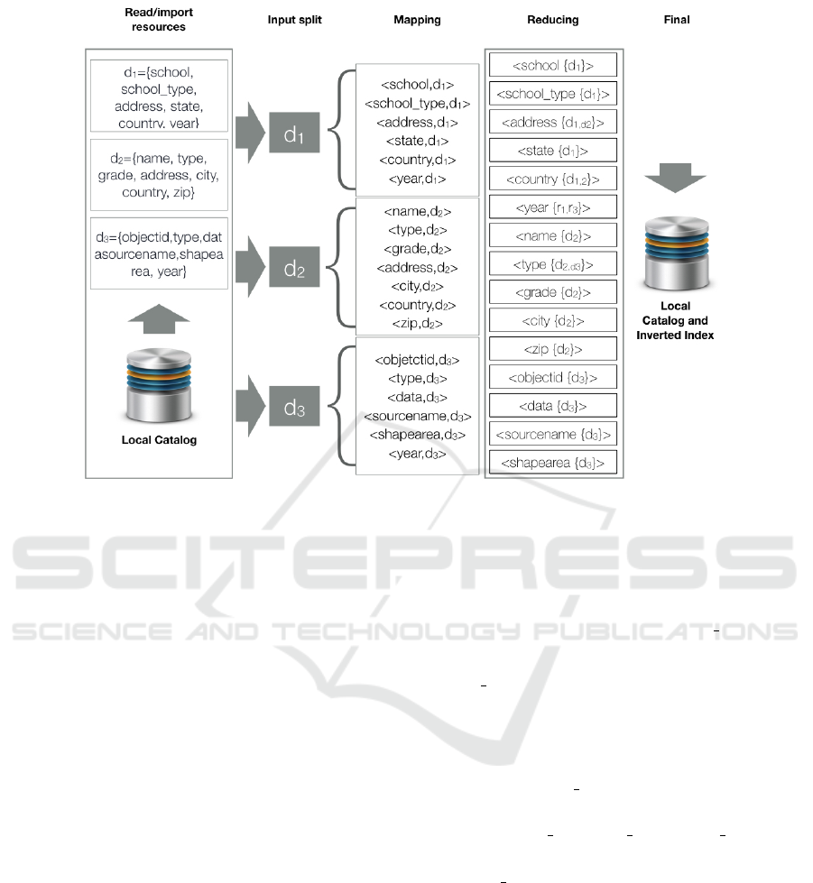
Figure 3: Building the Inverted Index for three open data sets by applying the Map-Reduce approach.

3.1 Crawler

This component gets information about the data sets

contained in the corpus published by an open data

portal and builds the local catalog. Figure 2 is use-

ful to clarify.

The crawler has been designed to connect with

several platforms usually adopted to publish open

data portals. Depending on the platform, the crawler

relies on a speciﬁc connector. Several connectors

were built, but, in particular, the most useful ones are

the following: the CKAN Connector, for the standard

platform named Comprehensive Knowledge Archive

Network; the Socrata Connector, for Socrata Open

Data Portals. Since these platforms are the ones

mostly used to build open data publishing services,

our prototype is ready to connect with a large vari-

ety of different open data services. Nevertheless, it is

easy to extend the crawler with new connectors.

3.2 Indexer

The Indexer builds the Inverted Index IN. This is ex-

ploited by the technique presented in Section 2.2, to

perform the VSM Dataset Retrieval. In the Hammer

prototype, the Indexer component extracts terms and

labels from schema and meta-data of each open data

set in the corpus C. The indexer creates an inverted

index of terms and labels, i.e., a data structure that

implements a function

TermWeighForDataSets : t → {ods id, w}

(1)

that, given a term t, returns a set of pairs denoting

the ods id of the data set and the weight w (number

between 0 and 1)

Within Indexer we adopted the Map-Reduce tech-

nique; for each data set and for each label in the

schema and in the meta-data, the map primitive gen-

erates a pair <t, ods id>. Then, the reduce primitive

transforms the set of pairs into a nested structure

IN= { <t,ods list: { ods id

, . . . , ods id

}> }

where ods list is the list of ids of data sets for which t

is a label in schema or in meta-data. This structure is

the inverted index IN.

Finally, the inverted index IN is stored into the lo-

cal database.

The advantage of using the Map-Reduce approach

is that it natively implements map and reduce primi-

tives in a distributed environment, thus permitting to

distribute the computation among several servers.

Figure 3 shows how the process works. Suppose

three open data sets labeled d

, d

and d

are in the

corpus C. Their schema appear in the upper left side

of the ﬁgure. The map primitive generates the set of

The Challenge of using Map-reduce to Query Open Data

335

Figure 4: The Retrieval Process.

tuples that describe each data sets. These tuples are

reported in the central part of the ﬁgure. Recall that

each tuple associates a term, in this case a property

name, with the data set identiﬁer. Finally, the reduce

primitive fuses all tuples with the same label: we ob-

tain the nested structures reported on the right hand

side of the ﬁgure, i.e., the inverted index IN.

3.3 Query Engine

At query time, the Query Engine exploits the inverted

index IN to retrieve the list of data sets relevant for

the query (it is better to say: for each neighbor query

nq ∈ Q).

Figure 4 depicts how the query engine works: it

receives the query and generates the set Q of queries

to process. Then, by exploiting the catalog and the

inverted index IN, it determines relevant data sets

and then provides (as output) the items within those

data sets that satisfy at least one selection condition

nq.sc of a query nq ∈ Q. Thus, the Query Engine

must implement all the steps of the retrieval tech-

nique introduced in Section 2.2. However, steps from

1 to 3, i.e., from query assessment to query expan-

sion, are not suitable for parallelization with Map-

Reduce, because they strongly rely on the compu-

tation of the Jaro-Winkler string similarity measure

(Cohen, 1998). These steps are implemented by a

single-thread process.

In contrast, step 4 (VSM Dataset Retrieval), Step

5 and Step 6 can be implemented by exploiting again

the Map-Reduce approach.

• Step VSM Dataset Retrieval and Step Schema Fit-

ting determine, for each neighbour query nq ∈ Q,

the list of relevant data sets, i.e., those data sets

which items of interest for the user are likely to

be extracted from. To this end, a relevance mea-

sure rm for a data set ods w.r.t. a neighbour query

nq is deﬁned as:

rm(ods, nq)=

(1 − α) × krm(ods, nq) + α × sfd(ods, nq)

krm(ods, nq) is the Keyword-based Relevance

Measure, i.e., the relevance of a data set on the

basis of relevant keywords in query nq; sfd is the

Schema Fitting Degree, i.e., a measure between 0

and 1 that evaluates if the schema of the data set

ods is suitable for the query nq. α ∈ [0, 1] is a pa-

rameter that permits to balance the contribution of

both krm and sfd to the overall relevance measure.

The outcome of this step is the set RD= {ods

} of

relevant data sets.

• For each ods

∈ RD, Instance(rd

) is collected

from the open data portal and temporarily stored

into the local storage.

• The result set RS of relevant items is obtained by

evaluating the selection condition provided with

the neighbour query nq for which the data set was

retrieved. Again, the Map-Reduce approach is a

good solution to deal with heterogeneous items in

a parallel way.

The keyword-based relevance measure

krm(ods, nq) is computed by adopting the vec-

tor space model approach.

Consider a neighbour query nq ∈ Q (where Q is

the set of queries to process): its set of keywords

K(nq) can be represented as a vector v = <k

, . . . ,

>. The vector w(nq) = <w

, . . . , w

> represents

the weight w

of each term k

in the set of keywords

K(nq); this weight is conventionally set to 1, i.e.,

= 1 (but different settings could be deﬁned, de-

pending on the role of each term in the query).

Given a data set identiﬁer ods id, vector

W(ods id)= <w

,. . . ,w

> }

is the vector of weights of each keyword k

for data set

identiﬁed by ods id, as obtained by evaluating func-

tion TermWehighForDataSetrs through the inverted

index IN.

The Keyword-based Relevance Measure krm(ods,

nq) for the data set ods (identiﬁed by ods id) w.r.t.

query nq is the cosine of the angle between vectors

w(nq) and W(ods id). The maximum value of rm

1, obtained when the data set is associated with all the

keywords, while values less than 1 but greater than 0

denote partial matching. A minimum threshold th is

used to discard less relevant data sets and keep only

those such that rm(ods, nq) ≥ th.

For each relevant data set, the Query Engine

downloads its instance from the Open Data Por-

tal. Instances are stored into a collection within the

KomIS 2017 - Special Session on Knowledge Discovery meets Information Systems: Applications of Big Data Analytics and BI -

methodologies, techniques and tools

336

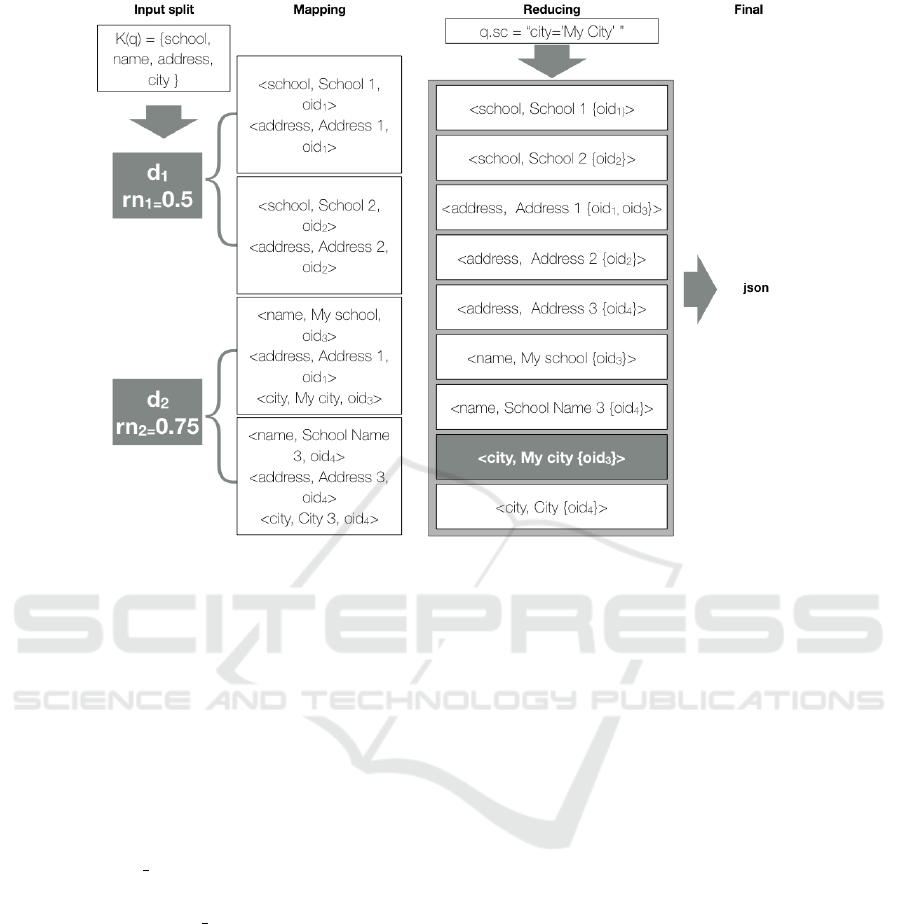
Figure 5: Retrieving relevant items by applying Map-Reduce.

NoSql MongoDB database. This way, we exploit the

schema-less feature of MongoDB, since the actual

schema of each retrieved data set can be very different

from each other. Instead, MongoDB is very useful to

manage heterogeneity.

Map-Reduce is exploited to select items as well.

First of all, the Query Engine assigns a unique iden-

tiﬁer to each item within the downloaded data sets.

In order to deal with heterogeneity of these objects

and easily select them, for each item and each ﬁeld

(property) in the item, the map primitive generates a

triple <oid, f ield value>. Then, the reduce primitive

transforms the set of triples into a nested structure

{ < f ield, value, oid list: { oid

, . . . , od

in order to aggregate all items having the same value

for a given ﬁeld.

To illustrate, consider a query q. Figure 5 il-

lustrates the process. Based on the set of key-

words K(q), we match two data sets d

and d

that

have sufﬁcient relevance w.r.t. the minimum thresh-

old th=0.3 (in Figure 5, rm

=rm(d

, nq)=0.5 and

=rm(d

, nq)=0.75)). Their instances are down-

loaded and items are processed by the map primitive

(see Figure 5). Then, the reduce primitive aggregates

triples based on the equality of ﬁeld name and value.

Finally, the items that match the selection condition

(in Figure 5, the gray item on the right-hand side) are

selected. In the example, only object with oid

is se-

lected.

4 EXPERIMENTS

We implemented our technique within the Hammer

prototype, so as to evaluate the effectiveness of the

technique and study performance. In this section, we

discuss execution times, to evaluate the effectiveness

of the Map-Reduce approach. Instead, the effective-

ness of the retrieval technique in terms of recall and

precision is reported in (Pelucchi et al., 2017).

4.1 Testbed

We assembled a testbed for evaluating the Hammer

prototype. It is a cluster of Hadoop nodes. We tested

it in two different environments: the ﬁrst one was on

local PCs and it was used for development and tuning;

the second environment was conﬁgured on Google

Cloud Platform and it was used to evaluate perfor-

mance in an industrial settings (i.e., with networking

connections having low latency and high throughput

during the download of datasets). Table 1 summarize

the different conﬁgurations of our tests.

Notice the three different conﬁgurations of the

Hadoop ecosystem: with 1 single node for storage

and computation; with 1 node for storage and 3 for

The Challenge of using Map-reduce to Query Open Data

337

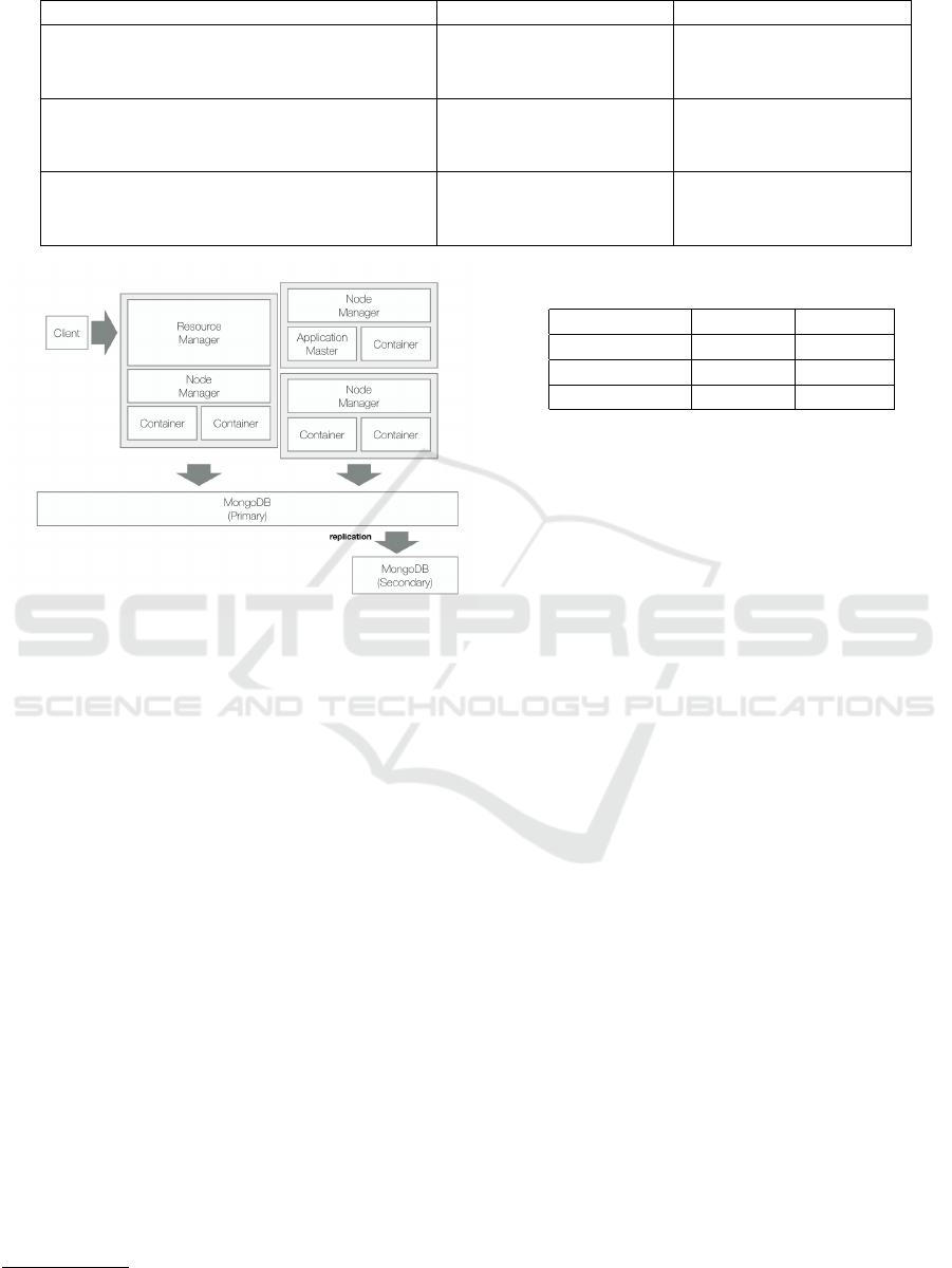
Table 1: Conﬁgurations of the Testbed.

Conﬁguration Storage Cluster

1. Single Node (Development CLuster)

1 Node

(1 virtual CPU

and 3 GB of memory)

1 Node

(1 virtual CPU

and 3 GB of memory)

2. Multiple Nodes (Development Cluster)

1 Node

(1 virtual CPU

and 3 GB of memory)

3 Node

(1 virtual CPU

and 3 GB of memory)

3. Multiple Nodes (Google Cloud Platform)

2 Node

(1 virtual CPU

and 3.75 GB of memory)

3 Node

(1 virtual CPU

and 3.75 GB of memory)

Figure 6: Architecture of the Prototype.

computation; (on Google Cloud Platform) with 5

nodes, 3 devoted to perform crawling, inverted in-

dex creation and query execution, 2 devoted to stor-

age (one node for the main instance of MongoDB and

one node hosting a replica). Figure 6 shows the archi-

tecture.

Experiments were performed on a set of 2301

open data sets published by the Africa Open Data por-

tal

. These open data sets are prepared in a non ho-

mogeneous way, as far as ﬁeld names and conventions

are concerned: Africa Open Data aggregates data sets

from a lot of different organizations. This fact makes

the search more difﬁcult than with an homogeneous

corpus: data sets are different by format, type and ar-

gument.

4.2 Crawling and Indexing

First, we tested crawling and indexing. The results

are reported in Table 2, for the three different conﬁg-

urations.

First of all, notice the execution times for crawl-

ing. A dramatic improvement is obtained by pass-

ing from conﬁguration 1 (one node) to conﬁguration

https://africaopendata.org/

Table 2: Response times (in sec) for crawling and indexing.

Conﬁguration Crawling Indexing

1 7524 972

2 3276 792

3 2448 774

2 (4 nodes), even in the development environment.

Then, conﬁguration 3 (on Google Cloud Platforms)

further reduces execution times. The overall gain is

from more than 2 hours to 40 minutes.

As far as indexing is concerned, increasing the

number of nodes is not particularly effective. In fact,

passing from conﬁguration 1 (one node) to conﬁgu-

ration 2 (4 nodes) we save 180 secs, i.e., the 18%.

In contrast, moving to conﬁguration 3 (Google Cloud

Platform), just a few seconds are saved. This is due

to the reduce primitives, that must aggregate sparse

tuples coming from the map primitive.

4.3 Querying

We run 6 different queries. They are reported in Fig-

ure 7. Hereafter, we describe them to help the reader

to understand what kind of queries it is possible to

perform.

• Information about nutrition in Kenya. In query

, we look for analytical information (number of

cases of underweight, stunting and wasting) about

malnutrition in the regions of Monbasa, Nairobi

and Turkana in Kenya.

• Civil unions statistics. In query q

, we look for

information about civil unions since 2012, where

the age of both spouses is at least 35. The at-

tribute extract are year, month, spouse1age and

spouse2age.

• Availability of water. Query q

retrieves in-

formation about availability of water, a seri-

ous problem in Africa; it looks for distribution

points that are functional (note the condition,

KomIS 2017 - Special Session on Knowledge Discovery meets Information Systems: Applications of Big Data Analytics and BI -

methodologies, techniques and tools

338

Table 3: Time of execution in seconds for each steps of the querying process.

Conﬁguration 1

Query

Assessment

Keyword

Selection

Neighbour

Queries

VSM Data

Set Retrieval

Schema

Fitting

Instance

Filtering

Total

time

107 10 529 1535 7740 6 9927

114 11 257 576 8453 2410 11821

82 10 179 746 8156 5615 14788

61 14 313 609 8969 2414 12380

60 19 35 93 455 218 880

45 9 28 29 262 37 410

Conﬁguration 2

Query

Assessment

Keyword

Selection

Neighbour

Queries

VSM Data

Set Retrieval

Schema

Fitting

Instance

Filtering

Total

time

105 12 534 990 4967 3 6611

117 11 257 456 5624 1099 7564

91 13 165 707 4591 2577 8144

64 12 321 439 4086 1475 6397

61 21 32 47 203 95 459

34 11 37 20 139 21 262

Conﬁguration 3

Query

Assessment

Keyword

Selection

Neighbour

Queries

VSM Data

Set Retrieval

Schema

Fitting

Instance

Filtering

Total

time

98 9 433 895 2345 2 3782

99 7 212 432 2478 725 3953

87 9 134 654 1572 759 3215

59 7 291 321 804 1077 2559

48 11 21 23 159 48 310

21 6 23 15 82 12 159

where we consider two possible values for ﬁeld

functional-status (functional and yes).

• Public schools metrics. Query q

looks for in-

formation about the number of teachers in pub-

lic schools, for each county. The query returns

county, schooltype and noofteachers.

• Water consumptions. In query q

, we look for

data about per capita water consumptions at the

date of December, 31 2013 (the date is written as

"2013-12-31t00:00:00").

• National Export statistics of Orchids. Query q

retrieves data about orchids export in terms of

weight (ﬁeld kg) and money.

Tables 3 summarizes execution times in secs, re-

porting the details for each step described in Section

2.2. The table is divided in three groups, one for each

conﬁguration.

The Query Engine was conﬁgured with the fol-

lowing minimum thresholds: th= 0.3 is the minimum

threshold for data set relevance measure, th sim=0.8

is the minimum threshold for Jaro-Winkler (Cohen,

1998) string similarity metric (to build neighbour

queries) with up to three alternative terms for each

substituted term. This setting is the one (see (Peluc-

chi et al., 2017)) that obtained the best performance

in terms of recall and precision, but it is also the one

that retrieves the highest number of data sets. This is

why we adopted this setting to test execution times.

The reader can see that, at the current stage of de-

velopment, execution times are very long, in some

cases several hours (when thousands of neighbour

queries must be processed). In particular, a not efﬁ-

cient step is Schema Fitting, because the schema of a

data set retrieved by the VSM Dataset Retrieval must

be ﬁtted against all the neighbour queries. Currently,

this step is not optimized: we plan to do that in the

near future.

Instead, the execution time of step 6 Instance Fil-

tering strongly depends on the actual size of down-

loaded data set instances.

Number of neighbour queries generated for each origi-

nal query: 243 for q

, 562 for q

, 81 for q

, 91 for q

, 263

for q

and 9 for q

The Challenge of using Map-reduce to Query Open Data

339

:<dn=nutrition,

P= {county, underweight, stuting,

wasting},

sc= (county = "Monbasa"

OR county = "Nairobi"

OR county = "Turkana") >

:<dn=civilunions,

P= {year, month, spouse1age,

spouse2age},

sc= (year = 2012 AND (spouse1age >= 35

OR spouse2age >= 35) >

:<dn=wateravailability,

P= {district, location, position,

wateravailability} ,

sc= (functional-status = "functional"

OR functional-status = "yes" ) >

:<dn=teachers,

P= {county, schooltype,

noofteachers} ,

sc= (schooltype="public") >

:<dn=waterconsumption,

P= {city, date, description,

consumption per capita} ,

sc= (date = "2013-12-31t00:00:00") >

:<dn=national-export,

P= {commodity, kg, money} ,

sc= (commodity = "Orchids") >

Figure 7: Queries for the Experimental Evaluation.

Anyway, as far as the effectiveness of Map-Reduce,

the results are promising: both step 4 VSM Dataset

Retrieval and Step 6 Instance Filtering strongly re-

duce their execution time. Thus, we can expect that

a conﬁguration with a larger number of computing

nodes will better parallelize the execution and will ob-

tain faster response times. Finally, the reader can no-

tice that the conﬁguration on Google Cloud Platform

is always the oe with better performance: a better vir-

tual environment and an excellent network infrastruc-

ture speed up the prototype.

5 RELATED WORKS

The world of Open Data is becoming more and more

important for many human activities. Just to cite some

areas that can get beneﬁts, we cite Neuro-Sciences

(Wiener et al., 2016), prediction of tourists’ response

(Pantano et al., 2016) and improvements to digital

cartography (Davies et al., 2017). These works are

proving the concept of Open Data Value Chain: the

wide adoption of Open Data by researchers and ana-

lysts shows that the effort of public administrations is

motivated and must be carried on.

We now focus on Open Data Management re-

search. This area is young and in progress. In par-

ticular, at the best of our knowledge, our approach is

novel and no similar systems are available, at the mo-

ment. Anyway, some works have been done.

An interesting paper is (Braunschweig et al.,

2012), where the authors observe characteristics of

ﬁfty Open Data repositories. As a result, they sketch

our vision of a central search engine.

In (Liu et al., 2006), the authors note that there is

a growing number of applications that require access

to both structured and unstructured data. Such collec-

tions of data have been referred to as dataspaces, and

Dataspace Support Platforms (DSSP) were proposed

to offer several services over dataspaces. One of the

key services of a DSSP is seamless querying on the

data. The Hammer prototype can be seen as DSSP of

Open Data, while (Liu et al., 2006) proposes a DSSP

of web pages.

In (Kononenko et al., 2014), the authors re-

ported their experience in using Elasticsearch (dis-

tributed full-text search engine) to resolve the prob-

lem of heterogeneity of Open data sets from feder-

ated sources. Lucene-based frameworks, like Elas-

ticsearch and Apache Solr (see (Nagi, 2015)), are al-

ternatives to the Hammer prototype, but they usually

don’t retrieve single items satisfying a selection con-

dition.

In (Schwarte et al., 2011), the authors describe

their approach and their idea to build a pool of feder-

ated Open Data Corpora with SPARQL as query lan-

guage. However, we considered SPARQL only for

people that are highly skilled in computer science: our

query technique is very easy to use and it is designed

for analysts with medium-level or low-level skills in

computer science.

The beneﬁt of Map-Reduce approach are de-

scribed in (Dean and Ghemawat, 2010). In few

words, Map-Reduce automatically parallelizes and

executes the program on a large cluster of commod-

ity machines. In (Vavilapalli et al., 2013), the au-

thors present YARN Yet Another Resource Negotiator

and they provide experimental evidence demonstrat-

ing the improvements of use YARN on production

environments. YARN is the basic component within

Hadoop that handles the actual execution of the Map-

Reduce tasks.

6 CONCLUSION

In this paper, we present the current state of develop-

ment of the Hammer prototype, a testbed for a novel

technique to query corpora of Open Data sets. In par-

KomIS 2017 - Special Session on Knowledge Discovery meets Information Systems: Applications of Big Data Analytics and BI -

methodologies, techniques and tools

340

ticular, in this work we faced the challenge of paral-

lelizing many parts of the prototype by applying the

Map-Reduce approach, in order to evaluate the fea-

sibility of this Big Data approach in the area of Big

Open Data. Speciﬁcally, the Hammer prototype im-

plements the retrieval technique presented in (Peluc-

chi et al., 2017). We demonstrated that the adoption

of modern standard technology speciﬁcally designed

for big data management, such as Apache Hadoop and

MongoDB, can be effective in this context, in partic-

ular increasing the number of nodes in the Apache

Hadoop ecosystem, even though the retrieval tech-

nique produces a large number of rewritten queries

(neighbour queries) and several parts of the prototype

are currently not optimized.

As far as the effectiveness of the query technique

is concerned, i.e., evaluation of the capability to re-

trieve what users want, we refer to our previous work

(Pelucchi et al., 2017), in which the technique has

been extensively introduced and evaluated on a cor-

pus of open data sets. In that paper we showed that

the technique is actually effective, in particular in

comparison with a tool like Apache Solr, that is a

stand-alone search engine. We discovered that, al-

though Apache Solr behaves quite well, our technique

is capable of better focusing on data sets of interest;

furthermore, it extracts only items of interest (while

Apache Solr does not in a classic conﬁguration).

In the future work, we will optimize the imple-

mentation of many components of the Hammer proto-

type, in order to get near real time response times. In

particular, we plan to replace the native Hadoop im-

plementation with Spark on a Hadoop Cluster to ob-

tain dramatic improvement of performance (accord-

ing to (Zaharia et al., 2010), Spark is 10x faster then

Hadoop).

Finally, we will extend queries to provide com-

plex features such as join and spatial joins ((Bordogna

and Psaila, 2004)) of retrieved data sets. In particular,

we are considering, as a starting point, the concept of

query disambiguation, in order to improve the genera-

tion of neighbour queries; a work we are considering

as a starting point is (Bordogna et al., 2012). Fur-

thermore, we think that a post processing of results is

necessary, in particular when thousands of items are

retrieved. We think that useful operators could be de-

ﬁned, similar to those introduced in (Bordogna et al.,

2008).

Similarly, the adoption of NoSQL databases for

persistent storage of retrieved results could be use-

ful, since the Hammer prototype provides collec-

tions of heterogeneous JSON objects, possibly geo-

referenced. A good idea could be to integrate the

concept of blind querying and the Hammer engine as

part of the J-CO-QL query language (Bordogna et al.,

2017), which is able to query heterogeneous collec-

tions of possibly geo-tagged JSON objects, providing

high-level operators which natively deal with spatial

representation and properties.

REFERENCES

Bordogna, G., Campi, A., Psaila, G., and Ronchi, S. (2008).

A language for manipulating clustered web docu-

ments results. In Proceedings of the 17th ACM con-

ference on Information and knowledge management,

pages 23–32. ACM.

Bordogna, G., Campi, A., Psaila, G., and Ronchi, S. (2012).

Disambiguated query suggestions and personalized

content-similarity and novelty ranking of clustered re-

sults to optimize web searches. Information Process-

ing & Management, 48(3):419–437.

Bordogna, G., Capelli, S., and Psaila, G. (2017). A big geo

data query framework to correlate open data with so-

cial network geotagged posts. In International Con-

ference on Geographic Information Science, pages

185–203. Springer, Cham.

Bordogna, G. and Psaila, G. (2004). Fuzzy-spatial sql. In

International Conference on Flexible Query Answer-

ing Systems, pages 307–319. Springer.

Braunschweig, K., Eberius, J., Thiele, M., and Lehner, W.

(2012). The state of open data. In WWW2012.

Carrara, W., Chan, W. S., Fischer, S., and van Steenbergen,

E. (2015). Creating Value through Open Data. Euro-

pean Union.

Cohen, W. W. (1998). Integration of heterogeneous

databases without common domains using queries

based on textual similarity. In ACM SIGMOD Record,

volume 27, pages 201–212. ACM.

Cukier, K. (2010). Data, data everywhere: A special report

on managing information. Economist Newspaper.

Davies, T. G., Rahman, I. A., Lautenschlager, S., Cunning-

ham, J. A., Asher, R. J., Barrett, P. M., Bates, K. T.,

Bengtson, S., Benson, R. B., Boyer, D. M., et al.

(2017). Open data and digital morphology. In Proc. R.

Soc. B, volume 284, page 20170194. The Royal Soci-

ety.

Dean, J. and Ghemawat, S. (2008). Mapreduce: simpliﬁed

data processing on large clusters. Communications of

the ACM, 51(1):107–113.

Dean, J. and Ghemawat, S. (2010). Mapreduce: a ﬂexible

data processing tool. Communications of the ACM,

53(1):72–77.

Kononenko, O., Baysal, O., Holmes, R., , and Godfrey,

M. (2014). Mining modern repositories with elastic-

search. In MSR. June 29-30 2014, Hyderabad, India.

Liu, J., Dong, X., and Halevy, A. Y. (2006). Answering

structured queries on unstructured data. In WebDB.

2006, Chicago, Illinois, USA, volume 6, pages 25–30.

Citeseer.

The Challenge of using Map-reduce to Query Open Data

341

Manning, C. D., Raghavan, P., Sch

utze, H., et al. (2008).

Introduction to information retrieval, volume 1. Cam-

bridge university press Cambridge.

Nagi, K. (2015). Bringing search engines to the cloud using

open source components. In Knowledge Discovery,

Knowledge Engineering and Knowledge Management

(IC3K), 2015 7th International Joint Conference on,

volume 1, pages 116–126. IEEE.

Pantano, E., Priporas, C.-V., and Stylos, N. (2016). You will

like it!using open data to predict tourists responses to

a tourist attraction. Tourism Management.

Pelucchi, M., Psaila, G., and Toccu, M. (2017). Building a

query engine for a corpus of open data. In Proceedings

of the 13th International Conference on Web Informa-

tion Systems and Technologies - Volume 1: WEBIST,,

pages 126–136. INSTICC, ScitePress.

Schwarte, A., Haase, P., Hose, K., Schenkel, R., and

Schmidt, M. (2011). Fedx: a federation layer for

distributed query processing on linked open data. In

Extended Semantic Web Conference, pages 481–486.

Springer.

Vavilapalli, V. K., Murthy, A. C., Douglas, C., Agarwal,

S., Konar, M., Evans, R., Graves, T., Lowe, J., Shah,

H., Seth, S., et al. (2013). Apache hadoop yarn: Yet

another resource negotiator. In Proceedings of the

4th annual Symposium on Cloud Computing, page 5.

ACM.

Wiener, M., Sommer, F. T., Ives, Z. G., Poldrack, R. A., and

Litt, B. (2016). Enabling an open data ecosystem for

the neurosciences. Neuron, 92(3):617–621.

Zaharia, M., Chowdhury, M., Franklin, M. J., Shenker, S.,

and Stoica, I. (2010). Spark: Cluster computing with

working sets. HotCloud, 10(10-10):95.

KomIS 2017 - Special Session on Knowledge Discovery meets Information Systems: Applications of Big Data Analytics and BI -

methodologies, techniques and tools

342