An Optimal Control Problem Formulation for a State Dependent

Resource Allocation Strategy

Paolo Di Giamberardino and Daniela Iacoviello

Department of Computer Control and Management Engineering ”A. Ruberti”, Sapienza University of Rome,

Via Ariosto 25, 00185, Rome, Italy

Keywords:

Optimal Control, State-based Cost Function, Switching Control, Epidemic Models, HIV Model.

Abstract:

In this paper, the problem of optimal resource allocation depending on the system evolution is faced. A

preliminary analysis deﬁnes the global effort required in any subset of the system state space according to

needed or desired goals. Then, in the deﬁnition of the cost function, the control action is weighted by a

piecewise constant function of the state, whose different constant values are deﬁned for each subset previously

deﬁned. The aim is to weight the control according to the distinct conditions, so getting different solutions

in each state space region so to optimize the planned resources according to the global goal. A constructive

algorithm to compute iteratively the ﬁnal control law is outlined. The effectiveness of the proposed approach

is tested on a typical model of human immunodeﬁciency virus (HIV) present in literature.

1 INTRODUCTION

In a control problem formulation, the main attention

is given on the global performances of the system ac-

cording to the desired state or output behavior. There

are several cases in which the effort for the control

goal achievements must be taken into consideration

for a suitable, realistic and physically acceptable re-

sult, especially when optimality is also desired for

the time length of the control action. In fact, in such

cases, the containment of the control strength and the

problem of the resource limitations can be considered

together in the same way; this is usually performed

both by introducing constraints in the control and in

the ad hoc choice of the cost index in which the cost of

the control is suitable deﬁned. This is a classical prob-

lem that can be easily solved by means of the Pon-

tryagin minimum principle; in the obtained solution

the optimal control can present discontinuities (Hartl

et al., 1995) at unknown instants, due to the presence

of the constraints on the input amplitude.

Applications of optimal control techniques range

from economics to biology, mechanics, telecommu-

nications and so on (Jun, 2004), (C.Liu et al., 2008),

(Nguyen and Sorenson, 2009). For the minimum time

problems with linear steady state system, the opti-

mal solution is bang-bang type with a limited number

of switching points (M.Athans and Falb, 1996). In

(Pasamontes et al., 2011) it is proposed to control

a solar collector making use of a switching control

strategy, showing that also changes in the dynamics

can be handled in the contest of optimal control. Im-

pulsive switching systems are another class of hybrid

dynamical systems in which global optimal control

strategies are proposed (R.Gao et al., 2010); they are

characterized by abrupt changes at the switching in-

stants.

The problem of optimal resources allocation

may arise when dealing with competing alterna-

tive projects which share common resources; this is

the so-called multi-armed bandit problem that has

received much attention especially in economics,

(Asawa and Teneketzis, 1996). In this case, the prob-

lem relies in determining the best strategy, among a

set of possible ones, knowing the state of each phase.

The decision is made on the basis of a payoff, i.e. a

cost, associated to the action.

In general, when dealing with the optimal control

of switched systems, like for examplethe optimal tim-

ing control problem, switching cost index can be in-

troduced to take into account the changes in the con-

trolled dynamics. One of the characteristic of these

problems is that the systems involved present continu-

ous dynamics subject to external discontinuous input

actuated by a switching signal generator. Different

schemes can be proposed and the optimal control the-

ory applied to hybrid systems allows to determine the

control input that optimizes a chosen performance

186

Giamberardino, P. and Iacoviello, D.

An Optimal Control Problem Formulation for a State Dependent Resource Allocation Strategy.

DOI: 10.5220/0006477801860195

In Proceedings of the 14th International Conference on Informatics in Control, Automation and Robotics (ICINCO 2017) - Volume 1, pages 186-195

ISBN: 978-989-758-263-9

index deﬁned on the state trajectory of the system.

This leads to two possible sub-problems, the time op-

timization problem and the optimal mode-scheduling

problem (Ding, 2009). The former relies in ﬁnding

the optimal placements of switching times assuming

a ﬁxed switching sequence; the latter is the problem

of determining the optimal switching sequence of a

switched system.

The presence of (white) noise perturbations can be

also considered, as in (Liu et al., 2005); an interesting

aspect is that the control weights are indeﬁnite and the

switching regime is described via a continuous-time

Markov chain. It is proposed a near-optimal control

strategy aiming at a reduction of complexity.

Numerical problems arising when dealing with

optimal switching control are considered in (Luus and

Chen, 2004) where a direct search optimization pro-

cedure is discussed.

In this paper the problem of optimal resource al-

location is related to the real time system behavior

considering the total amount of resources, i.e. the in-

put constraint, ﬁxed, and acting on the cost function,

in particular on the weight of the input, in order to

change the total cost according to the operative con-

ditions. The idea is to replicate a planning scheme in

which the designer ﬁxes the relevance of the control

action according to the conditions and, consequently,

changes the politics of intervention making the con-

trol effort more or less relevant. For example, in a

economic contest, within a preﬁxed total amount of

resources (input constraint), the investment of more

or less budget for the solution of some problem can

be driven by some social indicator indexes, like un-

employment below or over a preﬁxed critical percent-

ages, or the national PIL lower or higher a preﬁxed

threshold which guarantees economic grown, or the

level taxation, and so on.

Then, a cost index in which the control action is

weighted by a spatial piecewise constant function of

the state is introduced, so that its value changes de-

pending on the current state. The effect is to get dif-

ferent cost functions, deﬁned over each state space re-

gion, which weight the control differently depending

on the region in which the system operates, in order to

implement, in the contextof the classical optimal con-

trol formulation, a state dependent strategy. Changing

the weight for the control for each distinct state space

region corresponds to give a different relevance to the

control amplitude action with respect to the other con-

tributions, mainly errors, in the cost function. The re-

sult is that planning the different constant weights for

the control reﬂects in allowing the control to use dif-

ferent amplitudes, clearly higher in correspondence to

lower costs and lower for higher costs.

While the system evolves remaining in the same

state space region, the solution of the optimal control

problem gives an optimal solution for the control ac-

tion. When, during the state evolution, the trajectory

crosses from one region to another, a switch of the

cost function occurs at the time instant in which the

state reaches the regions separation boundary. From

that time on, a different optimal control problem is

formulated, equal to the previous one except for the

input weight in the cost function.

This procedure is iterated until the ﬁnal state con-

ditions are reached. The overall control results to be

a switching one, whose switching time instants are

not known in advance but are part of the solution of

the optimal control problem, depending on the op-

timal state evolution within each region. This kind

of approach is different from the others previously

recalled; here, the discontinuous switching solution

does not arise either for the presence of switching dy-

namics, or for control saturation, but comes from the

particular choice of the cost index. The control strat-

egy changes since in the cost index it is assumed that

the control needs to be weighted differently bringing

to different strategies depending on the actual state

value. It can be referred as a real time state dependent

weight.

A ﬁrst use of a switching formulation for an op-

timal control problem is proposed in (Di Giamber-

ardino and Iacoviello, 2017), applied to a classical

SIR epidemic diffusion. The effectiveness of the pro-

posed approach is then here shown making use of a

biomedical example, the control of an epidemic dis-

ease, the immunodeﬁciency virus (HIV). The HIV

model proposed in (Wodarz, 2001) and modiﬁed in

(Chang and Astolﬁ, 2009) is adopted. The choice of

this example comes from the consideration that usu-

ally the medical and social interest for the presence

of an epidemic spread depends on the level of diffu-

sion of the infection, being considered in some sense

natural if it is lower than a physiologic level and be-

coming more and more relevant as the intensity of the

infection increases. Then, according to the present ap-

proach, a state dependent coefﬁcient that weights dif-

ferently the control depending on the number of the

infected cells is introduced, taking as state space re-

gion division the sets that correspond to a physiolog-

ical level, a high but not serious level and a very high

risk level. This corresponds to change the interven-

tion strategy depending on the varied conditions; as

already noted, the possible switching instants are not

known in advance but are determined on the basis of

the dynamic variables evolution and on the optimiza-

tion process.

In general, the introduction of a continuous state

An Optimal Control Problem Formulation for a State Dependent Resource Allocation Strategy

187

function as a weight in the cost index can be found

in (Behncke, 2000) for the case of SIR dynamics.

There, the feasibility of different control actions is in-

vestigated along with the possibility of introducing a

weight of the vaccination control depending on the

number of susceptible subjects; it is assumed the hy-

pothesis that vaccination at higher densities may be

less expensive and logistically easier. The continuous

weight tate space function brings to some additional

conditions, more than the usual ones of an optimal

control problem formulation, to be fulﬁlled.

The introduction of a spatial piecewise constant

function instead of a generic one as weight function

for the control brings back the problem formulation,

and then the problem solution, to a classical formu-

lation, except for the fact that the whole solution is

obtained composing the different local solutions com-

puted in each region in which the state trajectory

evolves.

The paper is organized as follows: Section 2 is

devoted to the description of the proposed approach,

based on an iterative optimal control computation

driven by the state values. In Section 3 some re-

calls on the HIV model and the control described in

(Chang and Astolﬁ, 2009) are given. Then, in Section

4 the proposed control strategy with the state depen-

dent cost index is applied to the HIV model. In Sec-

tion 5 the numerical results obtained for the case study

here considered are presented and discussed. Conclu-

sions and future work are outlined in Section 6.

2 PROBLEM FORMULATION

Starting from some brief recalls on the classical op-

timal control formulation, the proposed approach is

introuced and described.

2.1 Recalls on Optimal Control

Problem Formulation

In the optimal control theory, the following classical

minimum time problem is considered.

Given a generic dynamical system

˙x(t) = f (x(t), u(t)) (1)

with x ∈ ℜ

, u ∈ ℜ

, x(t

) = x

, where f ∈ C

with re-

spect to its arguments, and the q-dimensional inequal-

ity constraints on the control action

q(u(t)) ≤ 0 (2)

and assumed the cost index

J(u(t), T) =

L(x(t), u(t))dt (3)

in which the Lagrangian L(x(t), u(t)) : ℜ

n+m

→ ℜ

depends on the state as well as on the control, ﬁnd

the optimal values for the control (u

(t)) and the ﬁ-

nal time (T

), under the state constraint (1) and the

inequality constraint on the input (2), satisfying the

ﬁnal condition

χ(x(T), T) = x(T)− x

= 0 (4)

for a given x

∈ ℜ

, with χ ∈ C

, such that dim(χ) =

σ, 1 ≤ σ ≤ n+ 1.

As well known, once the constraints are given, the

obtained solution is optimal for the speciﬁc choice of

the cost function J(u(t), T). Changing such a func-

tion, also the solution changes. This means that the

choice of the function J(u(t), T) or, equivalently, of

the Lagrangian function L(x(t), u(t)) represents a cru-

cial aspect of the whole design procedure. In addi-

tion, their structure strongly affects not only the re-

sult but also the design procedure. In fact, usually,

a linear combination of linear or quadratic terms is

adopted for L, with constant coefﬁcients representing

the weight of each term in the sum, i.e. how much it

is important in the evaluation of the optimality of the

solution.

Such a structure is justiﬁed by the simplicity in

the problem formulation and in the computation of

the solution as well.

There are authors proposing richer formulations,

in which some of the weights for the input variables

can be taken as nonlinear functions of the state vari-

ables, in order to assign different relevance to the

control action depending on the operative conditions,

(Behncke, 2000). Clearly, this kind of formulation

introduces some additional conditions to be fulﬁlled

and the complexity in the computation of the optimal

control grows signiﬁcantly, requiring additional spe-

ciﬁc hypothesis on the system behavior.

The idea developed in the present work, and il-

lustrated in the next Subsection 2.2, is to maintain the

richness of the nonlinear state dependent weights and,

at the same time, to preserve the simplicity coming

from the use of linear/quadratic terms in the problem

formulation and solution.

2.2 The Proposed Approach

A generic quadratic function of u(t) in L(x(t), u(t))

depending on the state, can be written as u

P(x)u,

where P(x) represents the different weight of the input

as a function of the state and then of the operative

conditions.

In the proposed approach, which aims at simpli-

fying the optimal control formulation preserving the

richness of a state space dependent weight, the state

ICINCO 2017 - 14th International Conference on Informatics in Control, Automation and Robotics

188

space is divided into N subsets I

, such that ∪

i=1

ℜ

, each of them corresponding to different strategies

to be adopted. Therefore, the function P(x) is deﬁned

P(x) = Π

when x ∈ I

(5)

with Π

∈ ℜ

m×m

positive deﬁned m × m matrix, i =

1, . . . , N, where the entries of Π

are designed in order

to manage the input cost as the state changes.

Then, while x ∈ I

, the term u

u is used in the

Lagrangian L(x(t), u(t)) which can be rewritten as

(x(t), u(t) to put in evidence such dependency.

Once that in the optimal control problem formula-

tion no state dependent weight is esplicitely present,

the solution can be found according to the well known

approach which makes use of the Hamiltonian

(x, λ, u) = L

(x, u) + λ

f (x, u) (6)

where λ : ℜ → ℜ

, λ(t) ∈ C

almost everywhere, is

the n–dimensional multiplier function for the differ-

ential constraint given by the dynamics. Clearly, such

a formulation holds only when x ∈ I

Under the constraints (2) and (4), the optimal solu-

tion can be obtained solving the necessary conditions

given by

λ = −

∂H

(x, λ, u)

∂x



(7)

0 =

∂H

(x, λ, u)

∂u



∂q(u)

∂u



η (8)

q(u) = 0 (9)

η ≥ 0 (10)

0 = H (x(T), λ(T), u(T)) (11)

λ(T) = −

∂χ(x(T), T)

∂x(T)



ζ (12)

where η(t) ∈ ℜ

, η ∈ C

almost everywhere, ζ ∈ ℜ

and along with conditions (1), (2) and (4). The solu-

tion obtained holds until x(t) ∈ I

and it is optimal in

such a region. If the solution is such that the com-

puted trajectory goes outside the region I

entering

a contiguous region I

, then a new problem has to

be formulated with initial condition for the state as

the value on the boundary between the regions I

and

reached by the previously computed control, and

making use of the Lagrangian L

(x, u) and, then, of

(x, λ, u) in the necessary conditions.

The ﬁnal solution is obtained by concatenating all

the partial solutions computed.

Clearly, such a solution cannot be deﬁned as op-

timal since in this formulation it is not computed ac-

cording to a unique cost index, but it is optimal if re-

stricted to each state space region.

In order to better illustrate the proposed approach,

an example in the epidemiological ﬁeld is provided;

in this kind of problems, the classical medical ap-

proach makes use of thresholds to classify the severity

of the infection and then this can be used to modulate

the control weight in the cost index.

In next Section 3 the mathematical model of one

case study, the HIV infection, is brieﬂy introduced,

and the proposed procedure is used in Section 4.

3 THE MATHEMATICAL MODEL

OF THE SAMPLE SYSTEM

Many different models have been proposed to de-

scribe the HIV (human immunodeﬁciency virus); the

virus infects the CD4 T-cells in the blood of an HIV-

positive subject; when the number of these cells is

below 200 in each mm

the HIV patient has AIDS.

Models of the HIV generally consider the unin-

fected CD4 T-cells, the infected CD4 T-cells, the in-

fectious virus, the noninfectious virus and the im-

mune effectors, (Banks et al., 2006). In (Chang and

Astolﬁ, 2009) also the effects of cytotoxic T lym-

phocyte (CTL) are taken into account aiming at de-

termining a control that drives the patients into the

long-term non progression (LTNP) status, instead to

progress to the AIDS one. A simpliﬁed system is pre-

sented in (Joshi, 2002) where only the concentration

of CD4 T-cells and the concentration of the HIV parti-

cles are analyzed; in this case two different treatments

strategies are introduced in the differential equations.

Among all the proposed strategies, the policy using

two drug controls appears to be the best one, since it

reduces the number of virus particles, beyond the rise

of the number of uninfected CD4 T-cells, (Zhou et al.,

2014). The problem of the fast mutation of the HIV is

faced in (E.A.H. Vargas, 2014); this could cause resis-

tance to speciﬁc drug therapies; the model predictive

control shows the best performance among the ones

based on a switched linear system to a nonlinear mu-

tation model. In (Ding et al., 2012) it is suggested the

use of the fractional-order HIV model as a descrip-

tion more realistic than traditional ones, thus obtain-

ing very low levels dosage of anti-HIV drugs.

In this paper, the HIV model proposed in (Wodarz,

2001) and modiﬁed in (Chang and Astolﬁ, 2009) is

used. It will be shortly recalled hereafter. In the com-

plete model the state variables to be considered are:

• the uninfected CD4 T-cells, denoted by x

(t);

• the infected CD4 T-cells, denoted by x

(t);

• the helper–independent CTL, denoted by z

(t);

An Optimal Control Problem Formulation for a State Dependent Resource Allocation Strategy

189

• the CTL precursor, denoted by w(t): it provides

long term memory for the antigen HIV;

• the helper-dependent CTL, denoted by z

(t): it

destroys the infected cells x

(t).

The equations describing the relations among

these variables are

˙x

(t) = γ− dx

(t) − β(1− u(t))x

(t)x

(t) (13)

˙x

(t) = β(1− u(t))x

(t)x

(t) − αx

(t) +

−(p

(t) + p

(t))x

(t) (14)

˙z

(t) = c

(t)x

(t) − b

(t) (15)

˙w(t) = c

(t)x

(t)w(t) − c

(t)w(t) +

−b

w(t) (16)

˙z

(t) = c

(t)w(t) − hz

(t) (17)

where γ, d, β, α, p

, p

, c

, b

and h are the

models parameters whose numerical values are dis-

cussed in (Wodarz, 2001) and the control u(t) is as-

sumed bounded.

In (Chang and Astolﬁ, 2009) the Authors aim to

determine a control making use of equations (13)

and (14) only, through a simpliﬁed representation

in which the contribution of (15), (16) and (17) to

the (13)–(14) dynamics is reduced to an approxi-

mated near-equilibrium polynomial term. The pro-

posed modiﬁed model is

˙x

(t) = γ− dx

(t) − β(1− u(t))x

(t)x

(t) (18)

˙x

(t) = −βx

(t)x

(t)ut + π(x

(t)) (19)

with

π(x

(t)) = a+ Bx

(t) + Cx

(t) + Dx

(t) (20)

For sake of simplicity, in the sequel the model

(18)–(19) with position (20) will be assumed, with

the initial conditions denoted by x

) = x

1,0

and

) = x

2,0

As well known, in optimal control the central as-

pect is the deﬁnition of the cost index, that is what is

required to be minimized; in this case, the control ef-

fort and the number of infected subjects seem to be a

good choice.

Another aspect to be considered is the problem of

resources allocation especially when they are partic-

ularly limited. For example, in (Yuan et al., 2015)

this problem is faced when a limited quantity of vac-

cine has to be distributed between two non-interactive

populations; in that case, a stochastic epidemic model

is assumed.

Hereafter, the resource limitation is introduced by

a constraint as (2).

4 IMPLEMENTATION OF THE

PROPOSED APPROACH

The example introduced in previous Section 3 can be

effectively used to describe the proposed approach.

In fact, it is possible to deﬁne different strategies in

terms of control effort to be applied according to the

severity of the infection, measured by the number

(t) of infected cells. In other words, for sake of sim-

plicity, it is possible to ﬁnd three levels of necessity

of intervention; if x

(t) is below a certain threshold,

say ξ

, no actual infection is diagnosed and then no

intervention is required; then, deﬁned ξ

as the level

of infected cells over which the infection presents se-

vere effects, it is possible to choose two different ef-

fort in case of x

(t) ≥ ξ

is greater or lower than ξ

in the ﬁrst case a stronger action is required than the

one in the second case, and this requirement can be

introduced in the control design setting a lower cost,

i.e. weight, to the control if x

(t) ≥ ξ

and a higher

weight when ξ

≤ x

(t) < ξ

So, according to the procedure described in Sub-

section 2.2, the state space x = (x

)

is divided into

three regions:



x ∈ ℜ

: x

< ξ





x ∈ ℜ

: ξ

≤ x

< ξ



(21)



x ∈ ℜ

: x

≥ ξ



is the region in which no control action is needed;

is the region corresponding to the presence of the

infection while I

corresponds to a severe stadium of

infection.

Choosing the cost function

J(u(t), T) =

+ K

(t)x

(t)u(t) + K

(t)+

+P(x(t))u

(t)



dt (22)

with K

> 0, i = 1, 2, 3, the state function P(x(t)) can

be set as

P(x(t)) = Π

, x ∈ I

P(x(t)) = Π

, x ∈ I

(23)

P(x(t)) = Π

, x ∈ I

with Π

< Π

, so that the control can assume higher

values when the infection is severe (x ∈ I

), being

cheaper than in the case of x ∈ I

. As far as Π

concerned, its value is not relevant since when x ∈ I

no control action is required and then no control prob-

lem has to be formulated.

Assuming the nontrivialinitial conditions x

1,0

∈ ℜ

and x

2,0

≥ ξ

, x

∈ I

for a certain i > 1, the constraint

(4) can be rewritten as

χ(x(T), T) = x

(T) − ξ

= 0 (24)

ICINCO 2017 - 14th International Conference on Informatics in Control, Automation and Robotics

190

while the resources limitation, i.e. the control con-

straint (2), can be explicitly written as

q(u(t)) =



(t)





−u(t)

u(t) −U



≤ 0 (25)

U > 0, where the ﬁrst component represents the non

negativity condition while the second one is the upper

bound limitation.

To solve the problem the classical optimal control

theory is applied; the Hamiltonian in each region I

deﬁned as

(t), x

(t), λ

(t), u(t)) =

= K

+ K

(t)x

(t)u(t) + K

(t) + Π

(t) +

+λ

(t)(γ − dx

(t) − β(1− u(t))x

(t)x

(t)) +

(t)(−βx

(t)x

(t)ut + π(x

(t))) (26)

and then the necessary optimal conditions given in

Subection 2.2 assume the explicit expressions

(t) = −

∂H

∂x

= −K

(t)u(t) + dλ

(t) +

+β(1− u(t))x

(t)λ

(t) +

+βx

(t)λ

(t)u(t)

(t) = −

∂H

∂x

= −K

(t)u(t) − K

+β(1− u(t))x

(t)λ

(t) +

+βx

(t)λ

(t)u(t) +

−λ

(t)



B+ 2Cx

(t) + 3Dx

(t)



0 =

∂H

∂u

∂q

∂u

∂q

∂u

= 2Π

u(t)

(t)x

(t) + βx

(t)x

(t)λ

(t) +

−βx

(t)x

(t)λ

(t) − η

(t) + η

(t)

0 = η

(t)q

(u(t))

0 = η

(t)q

(u(t))

(t) ≥ 0

0 = H

(x(T), λ(T), u(T))

(T) = 0

(T) = −ζ

∈ ℜ

with condition (24) too.

After some computations, deﬁning the function

W(t) as

W(t) = x

(t)x

(t)(−K

− βλ

+ βλ

) (27)

the optimal control satisfying the necessary condi-

tions previously introduced can be expressed as

(t) =











0 if W(t) < 0

W(t)

2Π

0 <

W(t)

2Π

< U

U if

W(t)

2Π

> U

(28)

By integration, denoting with



, x

(t), x

(t), u

(t)



the solution obtained over the

time interval



, T



, it is also the optimal solution as

long as x(t) ∈ I

If x

∈ I

and x(t) ∈ I

∀t ∈



, T



, one

has that the solution is the whole optimal solu-

tion, which can be indicated with the superscript



, x

(t), x

(t), u

(t)





, x

(t), x

(t), u

(t)



, and





= ξ

. Otherwise, there exists a time instant

t = t

such that x(t

−

) ∈ I

and x(t

) ∈ I

, i 6= j. Then,

a new optimal control problem must be solved, with

the same conditions as the previous ones after the sub-

stitutions t

= t

, x(t

) = x(t

), and the index j instead

of i.

In the present case, being two the effective re-

gions, the optimal solution obtained in the ﬁrst of the

previous case necessarily means that i = 2. Other-

wise, the switching condition does hold for i = 2 and

j = 3 or vice versa.

The control computation ends at step k ≥ 1 when,

after a a priori unknownnumber k−1 ≥ 0 of switches,

the solution



, x

(t), x

(t), u

(t)



is such that x(t) ∈

∀t ∈



k−1

, T



and condition (24) is satisﬁed.

For k > 1, the whole solution is then given by con-

catenating the k partial ones, so getting a switching

solution with switching times t

, i = 1, 2, . . . , k−1 and

optimal time T

= t

It is important to stress that in the proposed ap-

proach the presence of switching instants depends on

the evolution of the state: no information can be avail-

able, even on their existence. The state dependent

switching conditions makes possible a different in-

terpretation; the control law computed following this

procedure can be regarded as a continuous time op-

timal control over a discrete time feedback update

of the control parameters. The optimal control can

be computed and applied until the state belongs to

the given region I

; crossing the regions boundary is

equivalent to an event driven discrete state feedback

which updates all the parameters, mainly the Π

, and

recompute a new optimal control over the new state

space region I

5 SIMULATION RESULTS

In this Section the results of some numerical simula-

tions are presented, showing the behavior of the pro-

posed control design approach making use of the HIV

model presented in Section 3. In all the simulations

performed, the parameters reported in Table 1, taken

from (Chang and Astolﬁ, 2009), have been used for

the model (18)–(19), along with the initial conditions

An Optimal Control Problem Formulation for a State Dependent Resource Allocation Strategy

191

1,0

= 0.2 and x

2,0

= 3.

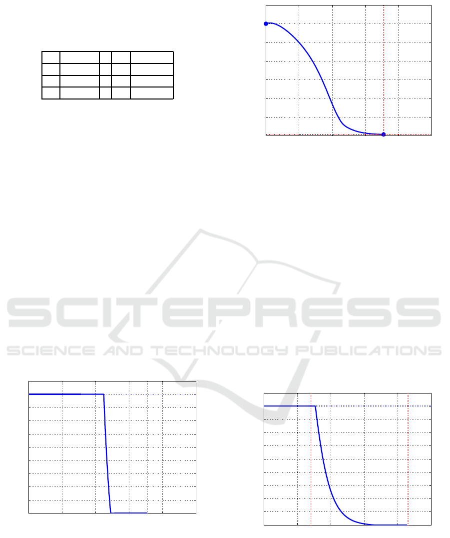
Table 1: Numerical values used for the HIV system param-

eters.

γ 1 B -3.1540

d 0.1 C 2.9402

β 1 D -0.6

α 0.0668

The choice of the HIV case study is quite meaning-

ful, since a switching control form takes the form

of a classical therapy strategy, being usually a piece-

wise constant control with the aforethought switching

times: it consists of a full drug dose for a limited time

and then a switch to zero, (Wodarz, 2001), sometimes

putting in evidence the daily therapy, (Chang and As-

tolﬁ, 2009).

An optimal control approach demands to the cost

function the ability to modulate the control accord-

ing to all the variables involved, possibly increasing

the performances of the control action. For a choice

of the cost index as in (22), the solution depends on

the values given to the weights assigned to each term.

In fact, in a classical minimum time optimal control

formulation, for the numerical choice of the constant

weights K

= 10, K

= 1 and K

= 20, taking for ex-

ample a constant weight P(x(t)) = P = 1 ∀x ∈ ℜ

, for

U = 0.9 as in (Chang and Astolﬁ, 2009) and ξ

= 0.03

in (4), the optimal control solution u

(t) obtained is

depicted in Figure 1, while Figure 2 reports the opti-

mal time evolution of the infected cells x

(t).

0 1 2 3 4 5

0.1

0.2

0.3

0.4

0.5

0.6

0.7

0.8

0.9

Time t

Optimal control u

(t): drug dose

Upper bound

Figure 1: Optimal control for constant input weight P = 1.

As expected, the choice of the weight for the input

u(t) in the cost index lower or equal to the ones as-

signed to the terms containing the infected cells pro-

duces an optimal control behavior equal to the upper

bound value from t

= 0 until the number of infected

cells is reduced at a level in which a high control ac-

tion is too expensive with respect to such a number,

0 1 2 3 4 5

0.5

1.5

2.5

3.5

Time t

Infected cells x

(t)

Figure 2: Infected cells evolution under optimal control.

and then it goes to zero as the x

(t) component de-

creases, so assuming a so called bang–bang behavior

between the upper and the lower bounds.

If the approach proposed in this paper is adopted,

the regions I

, I

and I

as in (21) must be introduced,

with their meaning discussed in Section 4, and with

the correspondingweights Π

as in (23) for the control

in the cost function (22).

The numerical values chosen are ξ

= 2, so that

the initial condition lies in the dangerous regionI

and

the solution must cross the normal region I

, Π

100 and Π

= 1, while Π

in this is not used due to the

no action region I

. The values for Π

and Π

with

≫ Π

have been chosen in order to signiﬁcantly

put in evidence the difference between a low cost, and

then a higher margin for the control effort and a high

cost, which should act against a high control effort.

0 1 2 3 4 5

0.1

0.2

0.3

0.4

0.5

0.6

0.7

0.8

0.9

Time t

Optimal control u

(t): drug dose

Upper bound

Figure 3: Full control for switched value of P(x(t)).

The solution obtained, depicted in Figure 3, is, con-

ﬁrming what planned, the concatenation of two seg-

ments; a ﬁrst optimal segment over the region I

the time interval 0 = t

≤ t < t

= 1.41, computed

with P(x(t)) = Π

, and then, at t = t

, the switch of

P(x(t)) from Π

to Π

produces the second segment

ICINCO 2017 - 14th International Conference on Informatics in Control, Automation and Robotics

192

which brings to the ﬁnal condition x

) = ξ

= 0.03

at time t = T

= 4.31.

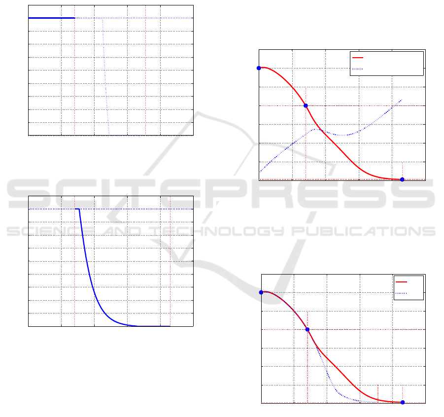
This composition of the whole control in the form

of a switching solution can be well put in evidence

plotting the solution obtained in the ﬁrst step of the

procedure, under the hypothesis that the state is con-

tained in the set I

, and marking the time instant t = t

in which the state trajectory reaches the boundary of

. This is done in Figure 4.

0 1 2 3 4 5

0.1

0.2

0.3

0.4

0.5

0.6

0.7

0.8

0.9

Time t

(t)

Upper bound

Figure 4: Optimal control obtained in the ﬁrst step of the

procedure, with the effective part from 0 to t

evidenced.

0 1 2 3 4 5

0.1

0.2

0.3

0.4

0.5

0.6

0.7

0.8

0.9

Time t

(t)

Upper bound

Figure 5: Optimal control obtained in the second step of the

procedure, with the effective part from t

to T

evidenced.

Then, in Figure 5 the solution of the optimal con-

trol problem deﬁned over I

starting from the initial

condition on its boundary corresponding to the value

reached in the previous phase is plotted. Comparing

the two Figures 4 and 5, it is possible to understand

the effect of the different weights of the input vari-

able on the control law obtained; in the ﬁrst case,

with a lower cost, the upper bound, i.e. the maximum

value, of the control is kept longer than in the second

case, being cheaper. In the second case, the cost of

the control forces the solution to reduce it as much as

possible to guarantee that the state reaches the ﬁnal

condition balancing the cost of the error with the one

of the control. The change of the control weight in

the cost function at the boundary between I

and I

produces a new behavior, characterized by a shorted

saturated action and a smoother decreasing shape, as-

suring, however, the convergence to the ﬁnal state.

The concatenation of the effective part in Figure 4

with the one in Figure 5 yelds Figure 3. Note that the

time instant in which the solution depicted in Figure

3 starts to decrease from the upper limit does not co-

incides with the switching instant t

: after the switch,

the control remains at its maximum but for less time

than in the non switching case.

0 1 2 3 4 5

0.5

1.5

2.5

3.5

Time t

Optimal state evolution

Infected cells x

tot

(t)

Uninfected cells x

tot

(t)

Figure 6: State evolution given by the full switched control.

The time history of the uninfected (x

(t)) and in-

fected (x

(t)) cells is depicted in Figure 6 where the

switching conditions and the corresponding time in-

stants are evidenced.

0 1 2 3 4 5

0.5

1.5

2.5

3.5

Time t

Infected cells x

(t)

tot

(t)

Figure 7: Time evolution of the infected cells in switched

and non switched case: a comparison.

A comparison between the evolution of the infected

cells obtained with the switching formulation and the

classical one coming from the use of a unique con-

stant value for the input weight is reported in Figure

7. Note that the non switching solution corresponds to

An Optimal Control Problem Formulation for a State Dependent Resource Allocation Strategy

193

keep P(x(t)) = Π

for all the state values, i.e. consid-

ering I

and I

as a unique region with a low cost for

the input, like in a standard optimal control problem

formulation. It can be noted that in the time interval

corresponding to the evolution in the I

region, the

solution, obtained using a low control weight only,

makes the state reach the ﬁnal condition faster and

keeps the number of the infected cells lower than in

the other case. Obviously, this is due to the fact that

the higher cost for the control brings the optimal con-

trol formulation to save the control effort, still bring-

ing to an effective solution as well.

Nevertheless, this apparent drawback is fully com-

pensated by the fact that the control, over the whole

time interval during which the drug is provided, re-

quires a lower contribution. This can be shown com-

puting and plotting the function

u(τ)dτ which give

a measurement of the total drug to be used in the ther-

apy.

Figure 8 is then obtained, showing that until both

solutions require the full control action (t = t

), up

to its bound, the functions are obviously coincident;

then, the decrement of the control in the switching

case, starting when the classical one is still at max-

imum, produces a reduction of the total amount of

input quantity, and then a reduced impact on the in-

fected patient and, at the same time, on the cost re-

lated to the therapy, despite its longer time of applica-

tion.

0 1 2 3 4 5

0.5

1.5

2.5

3.5

Time t

Time integral of the control u(t)

Switching solution

Classical non switching solution

Figure 8: Integral cost of the control action for the switching

solution and for the classical case: a comparison.

6 CONCLUSIONS

In this work a suitable non-linear cost index is as-

sumed in a minimum time optimal control problem

formulation, weighting the control by a state depen-

dent locally constant function. This approach can

deal with changes in the external conditions since it

is based on the state evolutions; it can tackle practi-

cal applications in telecommunications, biology, me-

chanics, economics, just to mention a few. The ef-

fectiveness of the proposed approach is veriﬁed con-

sidering a model of human immunodeﬁciency virus

(HIV) and proposing a cost index in which the con-

trol effort is weighted taking into account the number

of infected cells, giving higher attention when they

are dangerously over a ﬁxed critical value and con-

sidering the infection not much severe below. Obvi-

ously the result can be easily generalized to the case

of more than one critical value. The results obtained

show that this approach provides an efﬁcient resource

allocation, so being more effective, for example from

an economical point of view, than the classical theory

with the constant weight choice.

REFERENCES

Asawa, M. and Teneketzis, D. (1996). Multi-armed bandits

with switching penalties. IEEE Trans. On Automatic

Control, 41(3):328–348.

Banks, H., Kwon, H., Toivanen, J., and Tran, H. (2006). A

state-dependent riccati equation-based estimator ap-

proach for hiv feedback control. Optimal control ap-

plications and methods, 27.

Behncke, H. (2000). Optimal control of deterministic epi-

demics. Optimal control applications and methods,

21.

Chang, H. and Astolﬁ, A. (2009). Control of hiv infection

dynamics. IEEE Control Systems.

C.Liu, Gong, Z., Feng, E., and Yin, H. (2008). Opti-

mal switching control for microbial fed-batch culture.

Nonlinear analysis: Hybrid systems, 2.

Di Giamberardino, P. and Iacoviello, D. (2017). Optimal

control of sir epidemic model with state dependent

switching cost index. Biomedical Signal Processing

and Control, 31.

Ding, X. (2009). Real-time optimal control of autonomous

switched systems. PhD thesis, Georgia Institute of

Technology.

Ding, Y., Wang, Z., and Ye, H. (2012). Optimal control

of a fractional-order hiv- immune system with mem-

ory. IEEE Trans. On Control System Technology,

30(3):763–769.

E.A.H. Vargas, P. Colaneri, R. M. (2014). Switching strate-

gies to mitigate hiv mutation. IEEE Trans. On Control

System Technology, 22(4):1623–1628.

Hartl, R., S.P.Sethi, and Vickson, R. (1995). A survey of

the maximum principles for optimal control problems

with state constraints. Society for Industrial and Ap-

plied Mathematics, 37:181–218.

Joshi, H. (2002). Optimal control of an hiv immunology

model. Optimal control applications and methods, 23.

ICINCO 2017 - 14th International Conference on Informatics in Control, Automation and Robotics

194

Jun, T. (2004). A survey on the bandit problem with switch-

ing cost. The Economist, 152(4):513–541.

Liu, Y., Yin, G., and Zhou, X. (2005). Near optimal con-

trols of random-switching lq problems with indeﬁnite

control weight costs. Automatica.

Luus, R. and Chen, Y. (2004). Optimal switching control

via direct search optimization. Asian Journal of Con-

trol, 6(2):302–306.

M.Athans and Falb, P. (1996). Optimal Control. McGraw-

Hill, Inc., New York.

Nguyen, D. and Sorenson, A. (2009). Switching control for

thruster-assisted position mooring. Control Engineer-

ing Practice, 17.

Pasamontes, M., J.D.Alvarez, J.L.Guzman, Lemos, J., and

Berenguel, M. (2011). A switching control strategy

applied to a solar collector ﬁeld. Control Engineering

Practice, 19(2):135–145.

R.Gao, Liu, X., and Yang, J. (2010). On optimal control

problems of a class of impulsive switching systems

with terminal states constraints. Nonlinear Analysis,

73.

Wodarz, D. (2001). Helper-dependent vs. helper-

independent ctl responses in hiv infection: Implica-

tions for drug therapy and resistance. Journal theor.

Biol., 213.

Yuan, E., Alderson, D., Stromberg, S., and Carlson, J.

(2015). Optimal vaccination in a stochastic epidemic

model of two non-interacting populations. PLOS

ONE.

Zhou, Y., Yang, K., Zhou, K., and Wang, C. (2014). Optimal

treatment strategies for hiv with antibody response.

Journal of applied mathematics.

An Optimal Control Problem Formulation for a State Dependent Resource Allocation Strategy

195