Open Loop based Time Optimal PID Control Synthesis

Salim Bichiou, Mohamed Karim Bouafoura and Naceur Benhadj Braiek

LSA, Ecole Polytechnique de Tunisie, BP. 743, 2078 La Marsa, Tunisia

Keywords:

Minimum Time Control, Block Pulse Functions, PID Control, Optimization.

Abstract:

This paper deals with PID control tuning. The main objective being to minimize stabilizing/settling time of

linear control feedback. The presented method is based on an open loop time optimal control framework

reformulation into a closed loop system. Numerical tools such as orthogonal functions and optimization

algorithms are used to determine PID parameters that match a certain equivalent bang-bang control. Numerical

simulation of the obtained results shows the effectiveness of the proposed approach.

1 INTRODUCTION

Minimum time control has received a great attention

from researchers, this is particularly relevant since the

introduction of the maximum principe by (Pontryagin

et al., 1962). The methods used to solve such prob-

lems are numerous. Some of the approaches are ana-

lytical (shen et al., 2013) and are based on some afﬁne

mapping and graphical resolution. Others are numer-

ical (Lasserre et al., 2005) and uses computational

algorithms (Piccagli and Visioli, 2007) etc. Linear

systems minimum time control, due to the saturation

on both the input and output, feature a generalized

bang-bang solution. Speciﬁcally, the solution input

is a combination of bang-bang functions and linear

combination of modes associated to the zero dynam-

ics (Consolini and Piazzi, 2006).

On the other hand, researchers have used the or-

thogonal polynomials in many ﬁelds like tracking

control (Warrad et al., 2015) and model order reduc-

tion (Qi et al., 2014). Some have used them to solve

the minimum time control problem like the work pre-

sented in (Piccagli and Visioli, 2007). Where Cheby-

shev polynomials had been used to ﬁnd out the solu-

tion.

Furthermore, the orthogonal functions are a

widely used tool in the control ﬁeld. They have been

used for state estimation (Chou and Horng, 1986) and

used for systems that feature delays (Mohan and Kar,

2010). To ﬁnd a general solution for LTI system

with complex poles, orthogonal function were used

to solve the open loop problem (Bichiou et al., 2016).

In fact orthogonal function or polynomials like block

pulse functions (BPFs) are a powerful tool to solve

these problems numerically. It offers the advantage

of reducing the differential equations to a linear sys-

tem of algebraic equations through the use of the op-

erational matrix of integration and vector forms. It is

also noted that using piecewise orthogonal functions

such as block pulse instead of polynomial orthogonal

functions results in more relevant control. It captures

better discontinuities in the inputs (the control saught

is of type Bang-Bang).

In practice, one of the most popular control struc-

tures is the PID controller. This is due to its simplicity

and ability to achieve the desired performance with

various possible technologies (

Astr¨om and H¨agglund,

1995). In this paper a PID controller of a particular

structure (Pradhan and Ghosh, 2015) is adopted in or-

der to ﬁnd out the feedback signals that allows the

studied system to reach either its equilibrium state or

a desired steady state both in a minimum time.

Some issues in literature dealing with PID time

optimal control exists (Piccagli and Visioli, 2009). In

(Piccagli and Visioli, 2009), authors are interested to

derive a feedforward control for a closed loop system

with PID controller already designed. Then the objec-

tive is to improve the set-point following performance

of the controller. The system being constrained in

both input and output, so the open loop control is not

bang-bang.

In the proposed approach, we are basically search-

ing for PID parameters k

, k

and k

that permit to the

closed loop system to behave as it was controlled with

a minimum time bang-bang control.

The formulation of this problem, is mathemat-

ically simpliﬁed when using orthogonal function.

Then all system variables are expanded over that ba-

Bichiou, S., Bouafoura, M. and Braiek, N.

Open Loop based Time Optimal PID Control Synthesis.

DOI: 10.5220/0006433002790285

In Proceedings of the 14th International Conference on Informatics in Control, Automation and Robotics (ICINCO 2017) - Volume 1, pages 279-285

ISBN: 978-989-758-263-9

279

sis. Since then, in all the development, we will replace

states, output and control input with their coefﬁcients

when the development is truncated to a ﬁnite number

of functions.

Moreover, introducing, operational matrix of inte-

gration and some tensor properties could help us to

pose properly the basis of the framework.

The paper is organised as follows The second sec-

tion is reserved for the description of the used orthog-

onal functions and their algebraic properties. In the

third section, a formulation of the time optimal open

loop problem is given. The formulation of the opti-

mization problem and simulation results are presented

in the fourth section. In the ﬁfth section, a PID con-

troller structure is introduced. Discussion of the sim-

ulation results and discussion are shown in the sixth

section. Finally, concluding remarks and future works

are presented.

2 ORTHOGONAL FUNCTIONS

AND ALGEBRAIC

PROPERTIES

Using orthogonal functions (OF) to construct opera-

tional matrices was approached in the study of dy-

namic systems for modeling (Bouafoura et al., 2009),

identiﬁcation (Rao and Sivakumar, 1981); (Pacheco

and Steffen, 2002) and control purposes (Mohan and

Kar, 2010).

2.1 Function Development over OF

Principle

Any analytical function absolutely integrable on the

time interval [0, T] can be approximated as follows:

f(t) =

∞

∑

i=0

(t) (1)

where φ

(t) are the elementary orthogonal functions

and the coefﬁcients f

are evaluated by the following

scalar product:

f(t)φ

(t)dt (2)

For numerical purposes, a truncation of equation (1)

until a convenient number of elementary functions

must be done:

f(t)

∼

N−1

∑

i=0

(t) = F

(t) (3)

where Φ

= [φ

(t),φ

(t),··· ,φ

(t)] constitutes the

orthogonal basis and F

= [ f

, f

,· ·· , f

] is the co-

efﬁcient vector.

Integrating (3) transforms it as follows:

f(t)

∼

(t) (4)

where P

∈ R

n×n

is the operational matrix of integra-

tion depending on the considered orthogonal basis.

This approximation can ﬁt both orthogonal piece-

wise functions and orthogonal polynomials, in fact

their operational matrices in the integer case were

largely found out and applied in systems science.

As a result, the differential equations describing

dynamic processes can be reduced into algebraic re-

lations allowing important simpliﬁcations in the syn-

thesis problems.

2.2 Properties of the Block Pulse

Functions

Block pulse functions (BPFs) constitute a complete

set of orthogonal functions and are deﬁned over the

time interval [0,T] as follows (Wu et al., 2000):

(t) =







1 if t ∈ [iT , (i+ 1)T]

i = 0, ...,N − 1

0 otherwise

(5)

A function f (t) can be approximately represented by:

f(t) ≃

N−1

∑

i=0

(t) = F

φ(t) (6)

with

F = [ f

, f

,..., f

N−1

]

is the coefﬁcient vector.

φ = [ϕ

(t),ϕ

(t),...,ϕ

N−1

(t)]

is the block pulse ba-

sis vector.

is given by:

(i+1)T

f(t)φ

(t)dt (7)

where N is the dimension of the operational matrix.

The operational matrix for the block pulse functions

is given as follows:







1 1 ... 1

1 ... 1

.. . 1

0 .. . ... 0







(8)

3 TIME OPTIMAL OPEN LOOP

PROBLEM

In this part, a general minimum time problem is for-

mulated for SISO linear time invariant systems.

ICINCO 2017 - 14th International Conference on Informatics in Control, Automation and Robotics

280

We are particularly interested with the class of

systems described by:



˙x(t) = Ax(t)+ Bu(t)

y(t) = Cx(t)

(9)

where x ∈ R

is the vector of states, u ∈ R

is the

control input and y ∈ R

is the output.

The objective here is to determine the controller

sequence that allows the system to move from a

known point A to another point B in the least possible

time. For this, time optimization is required. That

leads to minimizing this cost function (Kirk, 1970):

J =

dt (10)

Applying The Pontryagin Maximum Principle (PMP)

(Pontryagin et al., 1962) and using the Hamiltonian

(Kirk, 1970), the the following control is derived.

This can be written as follows:

u(t) =



min

, if λ

B < 0

max

, if λ

B > 0

(11)

Thus, the obtained control is bang-bang.

To determine the control we need to determine the

sign of λ which is the co-state vector.

We remind here that this solution of the minimum

time control problem is solved in open loop.

4 BPFs BASED OPTIMAL

CONTROL SOLUTION

4.1 Formatting of the Control Problem

Finding the minimum time solution for system (9)

means solving multiple differential equations which

is a very difﬁcult task. In order to make this problem

easier to solve, BPFs based approach is used.

Considering the system (9) written in state space

form, in order to derive the ﬁnal time, a variable

change is considered as follows:

t = τt

(12)

This transformation allows us to go from the time

domain t ∈ [0,t

] to τ ∈ [0,1], the system states

become:

x(t) = ˜x(τ) (13)

Notice that, the latter variable change lead to a con-

stant time interval [0,1], for the used series. Since,

the ﬁnal time t

is unknown, we deduce,

˙x(t) =

d ˜x(τ)

dτ

˜x(τ) (14)

The original system (9) is now equivalent to:

˜x(τ) = A˜x(τ) + B ˜u(τ) (15)

The use of orthogonal functions consists on develop-

ing both, system states and input over that base:

˜x(τ) =

· φ

(τ)

˜u(τ) = ˜u

· φ

(τ)

(16)

Furthermore, integrating equation (15) leads to

(

X(τ) −

X(0)) = A

(

X(σ))dσ + B

˜u(σ)dσ

(17)

Introducing, coefﬁcients of ˜x(τ), ˜u(τ) and operational

matrix of integration we obtain:

X(σ)dσ =

(σ)dσ =

(τ) (18)

then we can write:

(

−

)φ

= t

+ B˜u

)φ

(19)

After the integration of equation (15) and the in-

troduction of coefﬁcients ˜x(τ),˜u(τ) (Bichiou et al.,

2016), we can write:

−

= t

+ B˜u

) (20)

where

depends on the chosen set of functions.

For the block pulse functions, the vector

is of the

following form:



X(0)

X(0) ···

X(0)



4.2 Optimization Algorithm

Consider the system model deﬁned in (9).

To ﬁnd the transition time from the initial position to

the target one need to solve the following nonlinear

problem (NLP):

min(t

)

(21)

subject to

˙x(t) = Ax(t) + Bu(t) 0 ≤ t ≤ t

u ∈ [u

min

max

]

x(0) = x

,x(t

) = x

(22)

then this problem is reported to the domain [0,1]. The

optimization algorithm in the orthogonalbase is of the

following form (OFNLP):

min (t f) (23)

subject to linear constraints:

˜u

Nmin

≤ ˜u

N,bp

≤ ˜u

Nmax

N f,bp



0 0 ·· · x



Open Loop based Time Optimal PID Control Synthesis

281

and nonlinear constraints:

−

= t

+ B˜u

) (24)

The resolution of such optimization problem can be

done through interior point routines like the function

”fmincon” implemented in Matlab. As a result the ﬁ-

nal time t

and the control sequence may be obtained.

5 SYSTEM WITH PID CONTROL

5.1 Closed Loop with PID

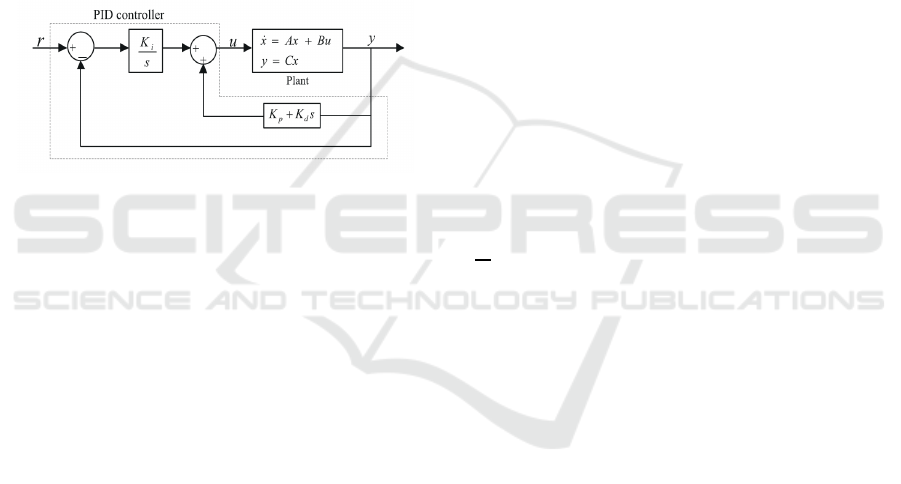
In this section, a PID controller is introduced to im-

prove the system performances. the considred feed-

back control is described by ﬁgure(1).

Figure 1: Feedback control structure.

the control effort is then given by:

u = k

Cx+ k

ξ+ k

C˙x (25)

where

ξ(t) =

(r− y)dτ (26)

In this work, we aim to ﬁnd the triplet {k

} that

steer the system from an arbitrary initial state to a

ﬁnal one. Hence, both stabilization and tracking may

be investigated.

Equation (25) could be written:

u = k

Cx+ k

ξ+ k

C(Ax + Bu) (27)

Then the control u becomes:

u = (1 − k

CB)

−1

Cx+ k

ξ+ k

C(Ax + Bu)] (28)

Let us note

K = [

] = (1− k

CB)

−1

Hence, in the following section, we are interested

to investigate

k, then pid controller gains could be

recovered as follows:

(1+CB

)

−1

(29)

(1−CB

) (30)

(1−CB

(31)

From the above, it is clear that ﬁnding PID controller

is possible iff both I − k

CB and I +CB

are invert-

ible. Moreover, in (Zheng et al., 2002), it is proven

that the existence of invertibility I − k

CB is neces-

sary and sufﬁcient for well-posedness of the MIMO

PID control problem.

5.2 PID Synthesis Formulation

In order to compute time optimal PID controller

gains, we propose ﬁrstly to consider the open loop

system and ﬁnd the optimal coefﬁcients of control ˜u

and system trajectory

. Let us denote ˜u

T∗

and

T∗

solutions of the optimization problem (OFNLP) pre-

sented in the last section.

The obtained control should obviously verify

equation (28):

˜u

T∗

−C

T∗

(32)

For numerical convenience, the latter expression of

the control should be introduced into the state equa-

tion with respect to the time domain of resolution.

Then it comes:

T∗

−

= t

T∗

+ B[

T∗

−C

T∗

) (33)

Rearranging equation (33), one may obtain:

(

T∗

−

)− A

T∗

= B





T∗

−C

T∗





(34)

Then

K could be found with the following formula:

vec(

K) = (F

⊗ B)

vec(G) (35)

with respect to the result (Brewer, 1978):

vec(XYZ) = (Z

⊗ X)vec(Y)

and where F is the last term of equation(34), while

G stands for the left hand side of the same equation,

⊗ denotes the Kronecker product (Brewer, 1978), vec

is the vectorization operator and (.)

is the Moore-

Penrose pseudoinverse of a matrix.

6 SIMULATION RESULTS AND

DISCUSSION

6.1 Example 1: Application to a Bridge

Crane

In this part, we intend to use the validated results on

a geometric model of a bridge crane (Ermidoro et al.,

2014).

ICINCO 2017 - 14th International Conference on Informatics in Control, Automation and Robotics

282

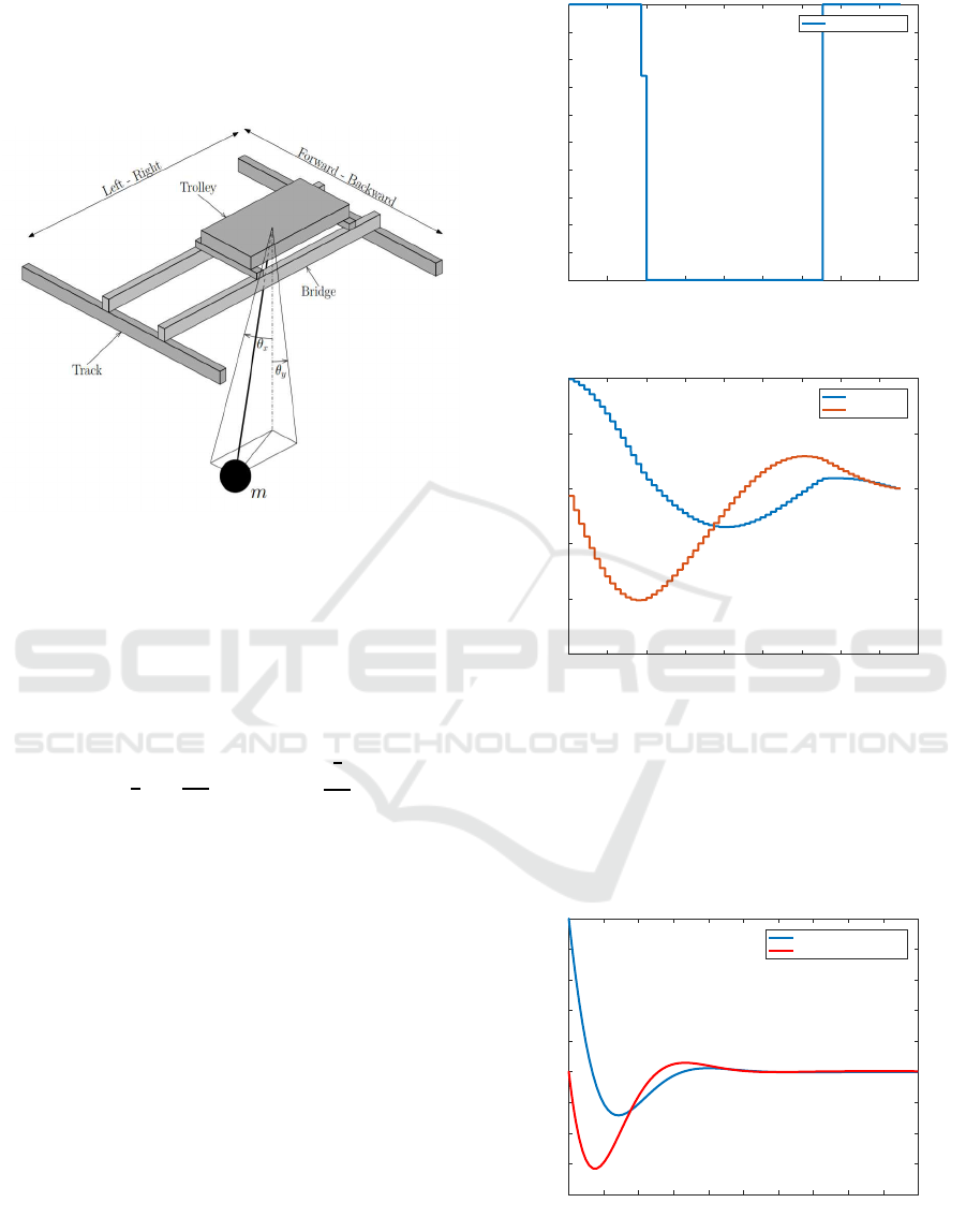
The system is composed of the bridge, moving

along the Y axis and the trolley, moving along the X

axis. The load is connected to the trolley by a rope

and can oscillate along any direction as described in

ﬁgure (2).

Figure 2: The typical structure of a bi-dimensional bridge

crane.

The model of the bridge crane is described by a

classical state space model:



˙x(t) = Ax(t) + Bu(t)

y(t) = Cx(t)

(36)

where

A =



0 1

−



B =



−



C =



1 0



(37)

Note that the control input is saturated and u ∈

min

max

The state vector x = [x

]

= [θ,

θ]

. We need

to move the system from x

= [θ

,0]

to x

= [0,0]

Hence, in this example, we assume that r = 0, The

system is shifted to its equilibrium point.

The physical parameters of the bridge crane are as

follows:

m = 1000kg,r = 5m, g = 9.81m/s

,b = 12000

The bounds of the controller is [−10,10]. As found in

(Ermidoro et al., 2014) for time optimal control t

4.2717s.

The control sequence of the system in open loop

when minimizing (OFNLP) is illustrated in ﬁgure (3).

The state trajectories of the system are given in

ﬁgure(4).

In this example, we deal with a stabilization prob-

lem, then we propose to use a previous result (Bichiou

et al., 2016) to obtain a state feedback gain. Then a

0 0.5 1 1.5 2 2.5 3 3.5 4 4.5

Time (s)

-10

-8

-6

-4

-2

Control sequence

Figure 3: Bridge crane control sequence in open loop.

0 0.5 1 1.5 2 2.5 3 3.5 4 4.5

Time (s)

-15

-10

-5

first state

second state

Figure 4: Bridge crane state trajectories in open loop.

method transforming that result to PID with the same

structure (ﬁgure 1) is applied (Pradhan and Ghosh,

2015).

The PID parameters are: k

= 488.7322, k

37.5069 and k

= 112.1876.

The system state trajectories are given in ﬁgure (5).

0 0.5 1 1.5 2 2.5 3 3.5 4 4.5 5

Time (s)

-8

-6

-4

-2

Closed loop first state

Closed loop second state

Figure 5: Bridge crane state trajectories using PID con-

troller.

Open Loop based Time Optimal PID Control Synthesis

283

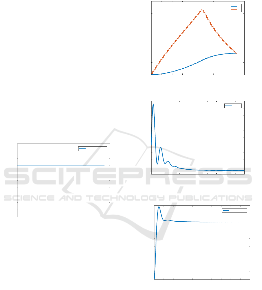
6.2 Example 2: Fighter Aircraft

In this part, we intend to use a linearized longitu-

dinal dynamics of the McDonnell Douglas Tailless

Advanced Fighter Aircraft (TAFA) (Kefferp¨utz and

Adamy, 2011) for tracking purposes.

The general representation of the system is of the

following form:



˙x(t) = Ax(t) + Bu(t)

y(t) = Cx(t)

(38)

where

A =



−1 1

6 −2



; B =





C =



0 1



(39)

with x

is the deviation of the angle of attack (rad) and

is the body axis pitch rate (rad/s).

The control variable is limited to |u| ≤ 20/180π

rad/s.

The system control is given in ﬁgure (6).

0 0.05 0.1 0.15

Time (s)

0.05

0.1

0.15

0.2

0.25

0.3

0.35

0.4

0.45

0.5

Control sequence

Figure 6: Fighter aircraft control in open loop.

The PID parameters are: k

= −0.6447, k

6.8510 and k

= 0.0064.

The state trajectories of the system are given in

ﬁgure (7).

The system control is given in ﬁgure (8).

The system output is given in ﬁgure (9).

7 CONCLUSIONS

In this paper, a based minimum time control prob-

lem for linear systems is proposed. In fact, the open

loop control determined with orthogonal function op-

timization is transformed to a PID controller. Hence,

dynamics of the closed loop system may be enhanced

and ﬁnal time could be reached in tracking as in a

classical bang-bang control. The whole development

0 0.1 0.2 0.3 0.4 0.5 0.6 0.7 0.8 0.9

Time (s)

0.2

0.4

0.6

0.8

1.2

Figure 7: Fighter aircraft state trajectories in open loop.

0 1 2 3 4 5 6 7 8 9 10

Time (s)

-0.2

-0.15

-0.1

-0.05

0.05

0.1

0.15

0.2

0.25

0.3

Control

Figure 8: Fighter aircraft PID control.

0 1 2 3 4 5 6 7 8 9 10

0.05

0.1

0.15

0.2

0.25

0.3

0.35

0.4

0.45

System output

Step Response

Time (seconds)

Amplitude

Figure 9: Fighter aircraft output with PID controller.

is carried with block pulse functions and related oper-

ational matrices. Simulations illustrate the validity of

the approach.

In future work, we intend to generalize the PID time

optimal control problem to some classes of nonlinear

systems.

ICINCO 2017 - 14th International Conference on Informatics in Control, Automation and Robotics

284

REFERENCES

Astr¨om, K. J. and H¨agglund, T. (1995). PID controllers:

Theory, Design, and Tuning. NC, second edition edi-

tion.

Bichiou, S., Bouafoura, M. K., and Braiek, N. B. (2016).

state feedback suboptimal time control method using

block pulse functions. In 24th Mediterranean Confer-

ence on Control and Automation (MED), pages 1224–

1229, Athens, Greece.

Bouafoura, M. K., Lanusse, P., and Braiek, N. B. (2009).

State space modeling of fractional systems using

block pulse fonction. In 15th IFAC Symposium on sys-

tem Identiﬁcation SYSID’2009, St Malo, France.

Brewer, J. (1978). Kronecker products and matrix calculus

in system theory. IEEE Transactions on Circuits and

Systems, 25(9):772–781.

Chou, J. and Horng, I. (1986). State estimation using con-

tinuous orthogonal functions. International Journal of

Systems Science, 19(9):1261–1267.

Consolini, L. and Piazzi, A. (2006). Generalized bang-

bang control for feedforward constrained regulation.

In 45th IEEE Conference on Decision and Control,

pages 893–898, San Diego, CA.

Ermidoro, M., Formentin, S., Cologni, A., Previdi, F., and

Savaresi, S. M. (2014). On time-optimal anti-sway

controller design for bridge cranes. In American Con-

trol Conference, pages 2809–2814, Portland, OR.

Kefferp¨utz, K. and Adamy, J. (2011). A tracking controller

for linear systems subject to input amplitude and rate

constraints. In American Control Conference, pages

3790–3795, San Francisco, CA.

Kirk, D. (1970). Optimal Control Theory: An Introduction.

Dover Books on Electrical Engineering.

Lasserre, J. B., Prieur, C., and Henrion, D. (2005). Non-

linear optimal control: Numerical approximations via

moments and lmi relaxations. In 44th IEEE Confer-

ence on Decision and Control, pages 1648–1653.

Mohan, B. M. and Kar, S. K. (2010). Orthogonal functions

approach to optimal control of delay systems with re-

verse time terms. Journal of the Franklin Institute,

347(9):1723–1739.

Pacheco, R. P. and Steffen, V. (2002). Using orthogonal

functions for identiﬁcation and sensitivity analysis of

mechanical systems. Journal of Vibration and Con-

trol, 8(7):993–1021.

Piccagli, S. and Visioli, A. (2007). Using a chebyshev tech-

nique for solving the generalized bang-bang control

problem. In 46th IEEE Conference on Decision and

Control, pages 4743 –4748, New orleans, LA.

Piccagli, S. and Visioli, A. (2009). Minimum-time feedfor-

ward technique for pid control. IET Control Theory

and Applications, 3(10):1341–1350.

Pontryagin, L. S., Boltyanskii, V., Gamkrelidze, R., and

Mischenko, E. (1962). The mathematical theory of

optimal processes. Interscience Publishers Inc, New

York.

Pradhan, J. K. and Ghosh, A. (2015). Multi-input and multi-

output proportional-integral-derivative controller de-

sign via linear quadratic regulator-linear matrix in-

equality approach. IET Control Theory and Applica-

tions, 9(14):2140–2145.

Qi, Z. Z., Jiang, Y. L., and Xiao, Z. H. (2014). Model order

reduction based on general orthogonal polynomials in

the time domain for coupled systems. Journal of the

Franklin Institute, 351(6):3200–3214.

Rao, G. P. and Sivakumar, L. (1981). Transfer function

matrix identiﬁcation in mimo systems via walsh func-

tions. In IEEE proc., volume 69, pages 465–466.

shen, Z., Huang, P., and Andersson, S. B. (2013). Calcu-

lating switching times for the time-optimal control of

singleinput, single-output second-order systems. Au-

tomatica, 49(3):1340–1347.

Warrad, B. I., Bouafoura, M. K., and Braiek, N. B. (2015).

Tracking control synthesis of nonlinear polynomial

systems. In 12th International Conference on Infor-

matics in Control, Automation and Robotics, pages

517–523, colmar, Alsace, France.

Wu, J. L., Chen, C. H., and Chen, C. F. (2000). A uni-

ﬁed derivation of operational matrices for integra-

tion in systems analysis. In International Conference

on Information Technology: Coding and Computing

(ITCC’00), pages 436–442, Washington, DC, USA.

Zheng, F., Wang, Q.-G., and Lee, T. (2002). On the de-

sign of multivariable pid controllers via lmi approach.

Automatica, 38(3):517–526.

Open Loop based Time Optimal PID Control Synthesis

285