
New Smith Predictor Controller Design for Time Delay System
Youcef Zennir, Mohand Said Larabi and Hassen Benzaroual
Automatic Laboratory of Skikda, Université 20 Août 1955, 26 route El-hadaiek, Skikda, Algeria
Keywords: Identification, Modelling, Time Delay System, IMC Controller, PID Controller, FOPID Controller, Didactic
Industrial System.
Abstract: This paper presents a robust control design based on Smith predictor and Fractional order PID (PID)
controller. This control technique has been used with other type of controllers (PID and IMC internal model
Controller) in order to ensure all performances required by several complex industrial process. Detailed
descriptions of the process with different mathematical models (with time delay) are exposed. One model is
validated around different operating points, by using different identification methods. We have used the
singularity function method to approximate fractional order in the FOPID structure. We have described
control principle’s and compare it with a different types of mentioned controllers in this study. Finally
several simulations have proved the efficiency of the new control design in term of stability, robustness and
precision.
1 INTRODUCTION
To be competitive, an industrial process must be
well controlled. Indeed, competitiveness requires
keeping process values as close as possible to its
required optimum performance and process
conditions: such as the products quality, production
flexibility, energy saving and safety of personnel,
facilities and the environment. The main role of
industrial controller is to keep the process under
control with the guarantee of a good dynamic and
static behaviour performance. Which can be
achieved by adjusting and adapting the transfer
function parameters in order to as close as possible
to the real process. In general, an industrial process
is modelled by a non-linear, linear (after
linearization) or linear mathematical model with a
time delay (Boyd, 1991). Regardless if these models
are stable or not are required a controller (control
action) to ensure the desired performance. The
objective of automatic regulation or servo-control of
a process is to keep the process values as close as
possible to its optimum of operating points,
predefined by the process specification (imposed
conditions or performance). Safety aspects of staff
and facilities should be taken into accounts, such as
those relating to energy and respect for the
environment. The specifications define qualitative
criteria to be imposed, which are usually translated
by quantitative criteria, such as stability, precision,
speed or evolution laws. Before going ahead and
develop the controller architecture and structure and
in case of unknown process parameters, an
identification phase is mandatory. Different
identification methods are existed in the literature
(Boyd, 1991; Ljung, 1999; Barraud, 2006). In our
study we are interested in the analogue flow control
system (Figure 1) by computing its mathematical
model via applying a different identification
methods (Broida, Strejc, etc.) and synthesis of its
control laws using several types: IMC, PID, FOPID
and Smith predictor controller and then at the end
we checked the simulation results with the process
experiments.
Figure 1: Experiment setup of a flow control (Abraham
and Denker, 2015).
598
Zennir, Y., Larabi, M. and Benzaroual, H.
New Smith Predictor Controller Design for Time Delay System.
DOI: 10.5220/0006426105980605
In Proceedings of the 14th International Conference on Informatics in Control, Automation and Robotics (ICINCO 2017) - Volume 1, pages 598-605
ISBN: 978-989-758-263-9
Copyright © 2017 by SCITEPRESS – Science and Technology Publications, Lda. All rights reserved
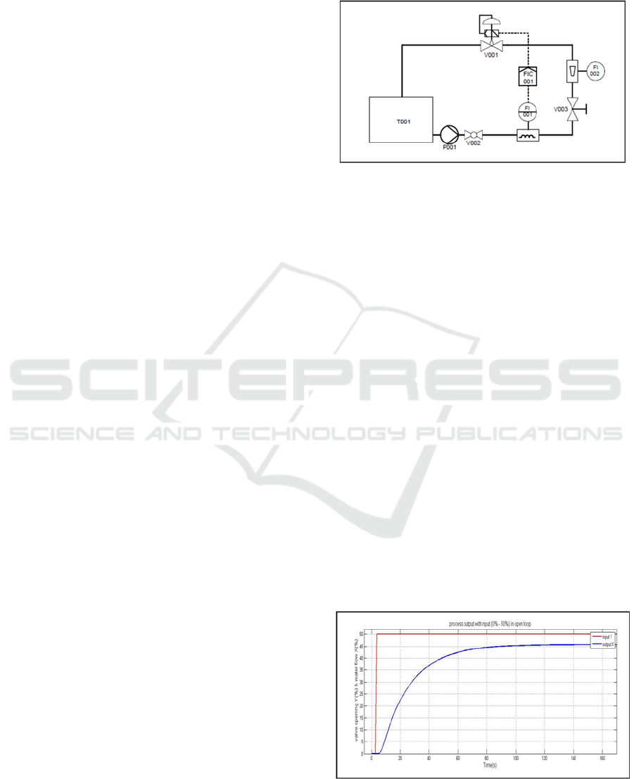
2 DIDACTIC INDUSTRIAL
PROCESS
The process illustrated in FIG. 1 consists of
numerous components and accessories (Abraham
and Denker 2015). The accessory components are
pre-installed on plates. The basic module offers a
large chassis for fast and safe mounting of the
respective required components of a test. The basic
module contains one storage tank: 75L (1),
Centrifugal pump (2), Compressed air controller
with pressure gage (0-2,5bar) with quick coupling
for supplying experiments (3), orifice with
Differential Pressure Sensor (Electro-pneumatic
control valve) (4), flow Rate Sensor
(Electromagnetic) (5), rotameter (6), valve (7) and
Switch cabinet (8). The Controlled System Flow is
operated with water as the working medium and
consists of a variable area flow meter. The flow
resistance can be configured using a valve (7), which
changes the flow properties in the controlled
systems.
One particular benefit of these controlled
systems is that, thanks to the float, all changes in the
flow rate caused by interference or behaviour of a
controller can be observed directly. The training
system has an electronic sensor with display for
measuring flow rates. It is suitable for measuring
flow rates of liquids in closed tubes. The
measurement variable is the flow rate. The ideal
flow velocity is 1-3m/s. The measurement principle
is electromagnetic induction according to Faraday's
law. Electromagnets or coils generate a magnetic
field, in which a conductor moves. This induces a
voltage. Here, the medium flowing in the flow rate
sensor corresponds to the moving conductor.
Therefore, for this type of measurement, a minimum
conductivity of the flowing medium is a
prerequisite.
The magnetic field is generated by pulsed direct
current of alternating polarity. The induced voltage
is proportional to the flow velocity and is tapped by
two measuring electrodes. The flow volume is
calculated from the flow velocity using the known
pipe cross-section. After a transformation there is a
standardized 4-20mA current signal proportional to
the flow rate available at the output. This sensor has
the advantage that flow resistances do not cause any
pressure drop, since it does not involve any moving
mechanical elements and the system's pipe cross-
section remains unchanged. The valves are
connected to the pipe system with PP-H plastic pipes
and clamp fittings or hoses. The closed loop flow
control diagram block, control with different
elements, which is represented by P&I diagram with
the follows figure (Abraham and Denker 2015). The
P&ID of flow control is presented as follows:
Figure 2: Flow control diagram (Abraham and Denker,
2015).
The identification methods used to identify our
process are described in the following section.
3 PROCESS IDENTIFICATION
The research of an industrial process model is
necessary in a model correctly representing the
process behaviour of the process. However, the
model must not be too sophisticated, at the risk of
being incompatible with the available corrector, or
be too simplistic not to mask certain aspects that are
detrimental to proper functioning. The choice of a
model, like its determination, must therefore be
judicious. The identification operation is carried out
in an open loop and this loop is no longer controlled
automatically. The controller is switched to manual
mode in order to act on the control signal. The
system can then be excited by a step signal with
different values. In principle, the output and input
must be of the same type with linear system (figure
3). If not, the system is nonlinear ((Ljung, 1999;
Barraud, 2006).
Figure 3: Process step response with input 0 % 50%.
New Smith Predictor Controller Design for Time Delay System
599
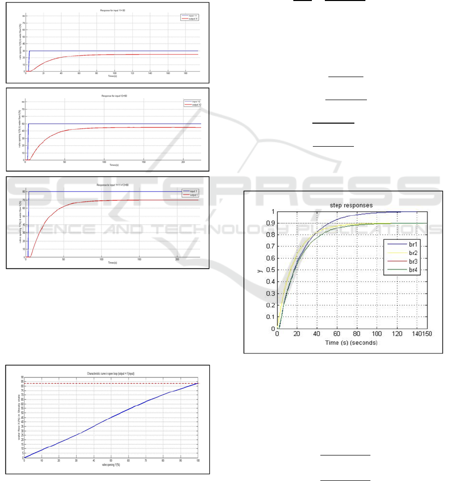
The figure 3 represents the system response to a
step input from 0% to 50%. We can see that the
output (flow measurement) converges towards the
input and that the system behaves us a first order
system with a certain time delay. In order to check
the linearity of the system, the used method is to
excite the system by two different steps inputs (0% -
30%) and (0% -50%), thus Y1 = 30% and Y2 = 50%
Y1 + Y2 = 80%, then the system was excited with
one input (0% -80%), shown in the follows figure:
Figure 4: Linearity proof of Process.
From Figure 4, we can see that the process has a
linear behaviour under certain operating conditions.
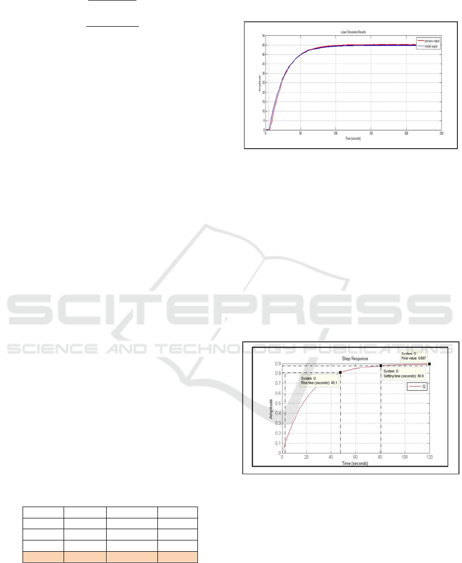
Using some several open-loop tests, the
characteristic curve, outputs = f (input) is
determined in steady state (figure 5).
Figure 5: Curve output=f(input).
The resulting curve (figure 5) is of the
substantially linear form, a straight line passes
through the origin Y=K * X, note that K represents
the system gain. The relation between flow rate and
opening of the valve is described by the following
equation: X (Y) ≈0.87 * Y. The mathematical model
of a stable process with a first-order model
behaviour and a time delay is described by the
following transfer function:
tf
s
Xs
Ys
K
T
∙s1
∙e
∙
(1)
Using Broida identification method and applying
these inputs (20% -84%), (0% -50%), (30% -50%)
(50%-70%) to the open loop. We have obtained the
following models:
Br
s
e
.
22∙s
1
(2)
Br
s
0.9
16.5∙s1
(3)
Br
s
0.9
19.25∙s 1
∙e
.∙
(4)
Br
s
0.85
16.5∙s 1
∙e
.∙
(5)
The step responses of the models are illustrated in
the following figure:
Figure 6: Linearity proof of Process.
In the second time we have used Strejc-Davost
identification method (Ljung, 1999), and we applied
the same inputs and the obtained the transfer
functions models: St
1
, St
2
, St
3
and St
4
respectively
are as follows:
St
s
e
.
9.07 ∙s1
(6)
St
s
0.9e
.
9.64 ∙s1
(7)
ICINCO 2017 - 14th International Conference on Informatics in Control, Automation and Robotics
600
St
s
0.9e
.
9.6∙s 1
(8)
St
s
0.85e
.
8.83∙s 1
(9)
4 IDENTIFICATION METHODS
We could identify our processes easily and, using
matlab function: ident command from the toolbox
identification. And we have obtained the dynamic of
the systems using input-output data from the
identified system. By following the follwing steps
are: Import of the data system, estimation and
validation of the model parameters. The Matlab
toolbox allows to identify a transfer functions, a
process models and the state space models, and also
provides an algorithms to evaluate the accuracy of
the identified models. We have used for each
operating point the data system of two tests carried
out under the same conditions (with the same inputs)
in order to estimate the model with the first test and
validate it with the second test. We have used as
well "Process model" method for model estimation.
The structure of this parametric estimation method is
a simple transfer function in continuous time which
describes a linear dynamic system. This model is
characterized by a static gain, time constant and time
delay. If some parameters are known, we need just
to enter their value and tick the box "Known". The
estimation algorithm will use these values for the
model. The behaviour of the system is close to the
first-order systems with a small time delay, so we
start from this point and we have made the
identification with the four datasets (same
measurement data used in the Broida or Strejc-
Davost identification methods). The general form of
the transfer function is given by (1).
The obtained models (transfer functions tf1, tf2,
tf3, tf4) with this method are illustrated in the
following table:
Table 1: Transfer functions with Ident (matlab).
Model K
p
T
p
T
d
tf1 0.92514 20.571 1.342
tf2 0.86879 19.891 2.541
tf3 0.91525 20.332 2.548
tf4 0.89686 20.539 0.5
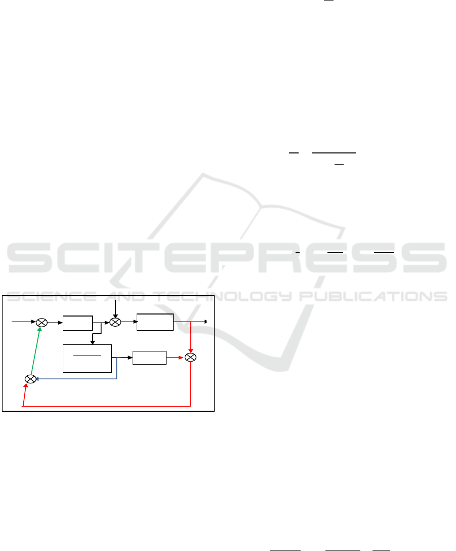
We have visualized the behaviour of the obtained
models with the different inputs and we have
compared the adjustment with the actual Best Fits
system. The obtained results are illustrated in the
following figures (response of the model described
by transfer function tf4):
Figure 7: Process step response with input 0 % 50%.
In the (figure 7) we could observe, that the
output process and model are very close to each
other after transitory regime. The following table
illustrates the best adjustments given by the models
with the different applied inputs. It is found that the
percentage of adjustment is always greater than
84.95%, with the model described by the tf4 transfer
function compared to the other models which give a
lower adjustment percentage.
Hence, we can say that tf4 is the model that
represents better the real system. The index response
of the open-loop model (tf4) is illustrated in the
following figure:
Figure 8: Step response of model tf4 in open loop.
The characteristics on open loop are not
satisfactory (the system is very slow, final value
different of 1) (figure 8). Hence we need to used a
controller to ensure the optimal characteristics and
improved the stability of process.
In the following section we use different
controllers in this study have been described and on
particularly the Smith’s predictor controller with
new structure.
New Smith Predictor Controller Design for Time Delay System
601
5 NEW DESIGN OF SMITH
PREDICTOR
In the literature, there are a large number of linear or
discrete linear controllers adequate for industrial
process control, which has linear system behaviour
(Kumar and Singh 2014). Among the most common
and most used controllers are PI, PD and PID with
different structures (Ali and Majhi, 2009). Also,
there is another type of controller that is more robust
than the conventional PID such as the internal model
controller (IMC) (Li et al., 2009; Wang et al., 2016;
Shamsuzzoha et al., 2012; Santosh kumar et al.,
2016; Xiao-Feng et al., 2016) and the Fractional
order PID controller (FOPID) (Bettou, 2011; Bettou
and Charef, 2008; Bouras et al., 2013).
Other types of controllers are developed
specifically to control systems with time delay such
as Smith's predictor (Shahri et al., 2014). This
controller was proposed for the first time by OJ
Smith in 1957 (Aidan and John, 1996; Resceanu,
2009).The main idea behind Smith's predictor is that,
since it is well known to correct systems without
time delay with a corrector (PID for example)
(Resceanu, 2009).
It does not correct the system without delay but
the output will then be estimated by delaying it by
the value of the system time delay. This very simple
approach leads to the following structure:
Figure 9: Smith predictor ( L=Td; Ks=Kp; =Td).
Different structures of Smith predictor has been
proposed in literature with different controllers. Note
that, the implementation of a Smith predictor
controller needs a very good model of the process.
In our study we have used only Fractional order PID
(FOPID) controller and with Smith predictor. The
structure type of the FOPID controllers is Fractional
order controller: PI
λ
D
. In control theory, the
conclusion about fractional control system is that it
can increase the stability region and robustness
(Esmaeilzade, 2014) moreover it gives performances
at least as good as its integer counterpart (Grimble,
2006). The transfer function of a FOPID controller,
which was initially proposed by Podlubny in 1999
(Esmaeilzade, 2014), is given by :
1
,
, 0
(10)
Where Kp, KI, KD R and , R+: are the
controller tuning parameters and the controller
design problem is to determine the suitable values of
these unknown parameters in such way it responds
to all control objectives (Grimble, 2006). Many
methods in literature have been proposed for FOPID
approximation (Bouras, 2013).
In this work we have used singularity function
approximation method of Charef (Bettou, 2011),
applied in FOPID controller. The fractional-order
integrator
,
∈
R+ is approximated as:
1
≅
1
,0
1,
∈
(11)
To have a good tuning parameters of the PI
D (Kc,
Ti , ) we have used the following algorithm
(Bouras, 2013) described in the steps below:
Step1: calculate the parameters
i
for 0≪i≪2
∙
∙
(12)
u
: the unit magnitude frequency of reference
model;
m: the derivation fractional order of the reference
model;
i
: calculated with the reference model parameters.
Step 2: calculate the parameters y
i
for 0≪i≪2
Using the following formulas:
∙
(13)
∙
∙
(14)
∙
∙
(15)
With y
i
: calculated from the transfer function Gp(s)
compared to the variable s at the point ωu; N:
samples number.
Step 3: calculate the parameters X
i
for 0 ≪i≪2
As per the following formulas:
.
(16)
C(s)
tf4(s)
e
-Ls
1
∙
r
u
y
d
Process
e
p
y
a
+
-
+
+
-
+
ICINCO 2017 - 14th International Conference on Informatics in Control, Automation and Robotics
602
.
.
.
(17)
With X
i
: derived from the controller transfer function
C(p).
Step 4: calculate the parameters K
c
, T
i
, with the
following formulas:
.
1
.
(18)
.
(19)
A comparative study is presented in the simulation
section between the various controllers cited before
in order to improve the performances of the process
and choose the best control suited for this type of
system.
6 SIMULATION
The simulation was done with closed loop and step
signal as input. Different diagram blocks has been
used with different controllers types. The simulation
time period equal 50s. We have used controller
Smith's predictor with IMC, PID, PI
λ
D
controllers.
We have applied an external and internal
perturbation (different time delay). The controller’s
parameters values are shown in the following tables:
Table 2: Parameters of Controllers.
Controlle
r
Kp
K
I
K
D
PID 10.5 0.808 1.87
PI
λ
D
10.5 147.3459 1.87
m==0.7
=1
The transfer function of the IMC controller is as
follows:
C
s
..
∙
.∙
∙.∙
.∙
∙
.∙
∙
(20)
The simulation is organized as below:
1. First study: Smith predictor controller with IMC
and PID controllers. Time delay equal 0.5 and
0.7. Perturbation applied after 25 s.
2. Second study: Smith predictor controller with
IMC or PID controllers, and FOPID controller.
Time delay equal 0.5s and 0.7s. Perturbation
applied after 25 s.
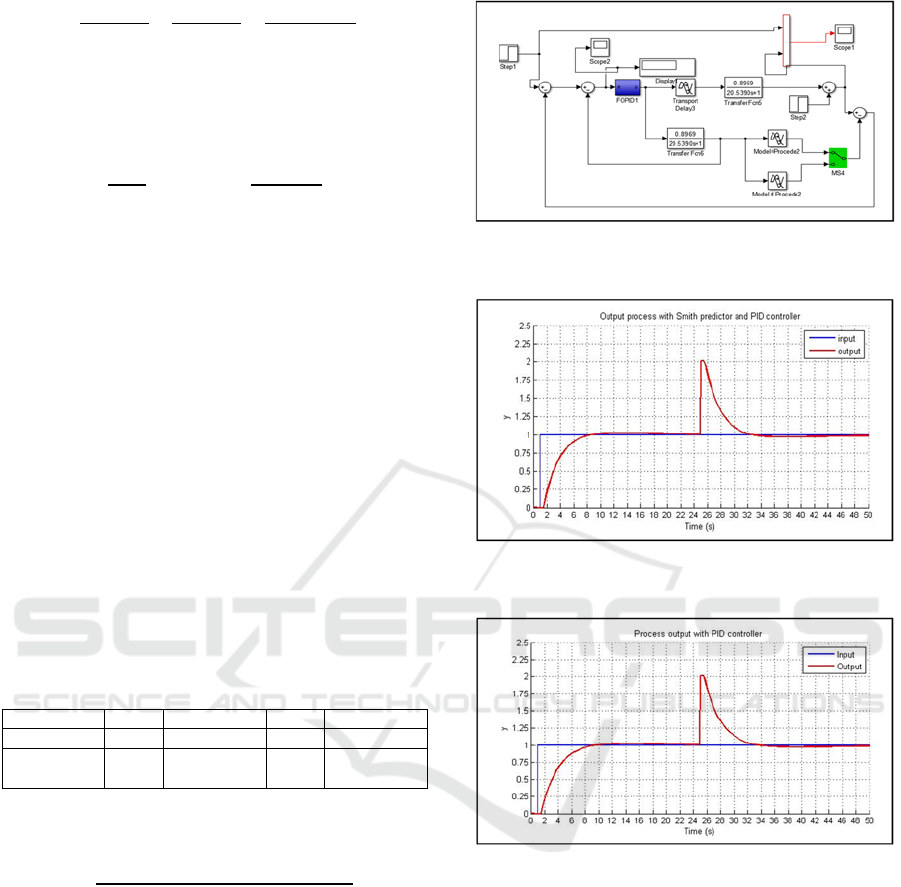
The block diagram of the control is as follows:
Figure 10: Block diagram of closed loop control with
Smith predictor and FOPID controller.
Figure 11: Input and Output curve (Process= model), with
Smith predictor and PID controller.
Figure 12: Input and Output curve (Process model, time
delay=0.7s), with Smith predictor and PID.
The obtained results illustrated by Fig.10, Fig11,
Fig.12 and Fig.13 show the PID controller is more
efficient (short response time) but IMC controller
give more precision. The obtained results illustrated
by Fig.14, Fig15, Fig.16, Fig.17, Fig.18 and Table
III shows the FOPID controller more efficient then
the PID and IMC (short response time and good
precision and stability).
New Smith Predictor Controller Design for Time Delay System
603
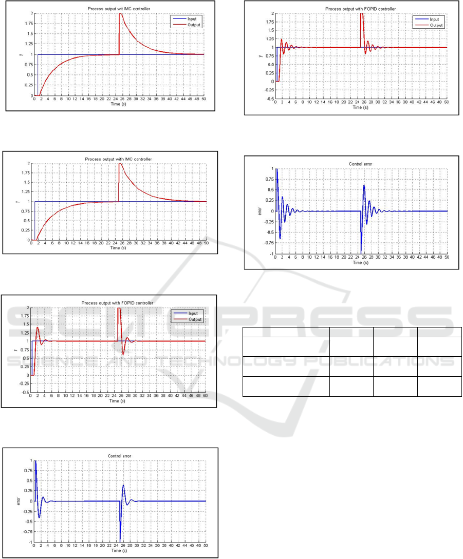
Figure 13: Input and Output curve (Process= model), with
Smith predictor and IMC controller.
Figure 14: Input and Output curve (Process model, time
delay=0.7s), with Smith predictor and IMC.
Figure 15: Input and Output curve (Process= model), with
Smith predictor and FOPID controller.
Figure 16: Error control (Process = model), with Smith
predictor and FOPID controller.
Figure 17: Input and Output curve (Process model, time
delay=0.7s), with Smith predictor and FOPID controller.
Figure 18: Error control (Process model, time
delay=0.7s), with Smith predictor and FOPID controller.
Table 3: Control error.
Control erro
r
PID IMC FOPID
Process=model
(time delay = 0.5s)
1.06.e
-2
-3.9.e
-3
2.42.e
-5
Process model
(time delay = 0.7s)
1.14.e
-2
-4.3.e
-3
2.48.e
-5
Process model
(time delay =5s)
5.2.e
-4
-3.1.e
-4
7 CONCLUSION
In this work we have presented the Smith Predictor
with IMC, PID and Fractional order PID controllers
applied to one of the industrial didactic process,
modelled by a linear model with time delay. A
detailed description of the system was presented
with different identification methods (Broida, Strejc)
used to obtain the best model. The chosen model has
been validated. And the obtained results show that
the new smith predictor structure with a Fractional
order PID control provides better performances to
the process compared with PID or IMC controllers.
And keep the study open for further optimization of
the FOPID parameters in case of a big time delay.
Different optimization algorithms can be applied
such as PSO or Genetic algorithms.
ICINCO 2017 - 14th International Conference on Informatics in Control, Automation and Robotics
604

REFERENCES
Abraham, D. and Denker, T. 2015. “Instruction Manual
RT 450 Modular Process Automation Training
System”. G.U.N.T. Gerätebau, Barsbüttel,
Germany,V. 0.1, p. 215.
Aidan, O. and John, R. 1996. “The control of a process
with time delay by using a modified Smith predictor
compensator”. Proceedings of the Irish Conference on
DSP and Control, Trinity College Dublin, pp. 37-44.
Ali, A. Majhi, S. 2009. "PI/PID controller design based on
IMC and percentage overshoot specification to
controller set point change". ISA Transactions, vol.48,
pp.10-15.
Barraud, J. 2006. “Control of processes with variable
parameters”. Mathematics. Ecole Nationale
Supérieure des Mines de Paris, p.161.
Bettou, K. 2011. "Analyse et réalisation de correcteurs
analogiques d'ordre fractionnaire", Mémoire de thèse,
Université de Constantine, p.111.
Bettou, K. Charef, K.A. 2008. "A New design method for
fractional PI
λ
D
μ
controller", IJSTA, vol.2(1), pp 414-
429.
Bouras, L. Zennir, Y. and Bourourou, F. 2013. "Direct
torque control with SVM based a fractional controller:
Applied to the induction motor". Proceeding of the 3rd
IEEE international conference on system and control
29-31 October. Algeria, pp.702-707.
Boyd, S. and Barratt C. 1991. “Linear Controller Design:
Limits of Performance”, Originally published by
Prentice-Hall, p.426.
Esmaeilzade, S.M., Balochian, S., Balochian, H., and
Zhang, Y., 2014. Design of Fractional–order PID
Controllers for Time Delay Systems using Differential
Evolution Algorithm. Indian Journal of Science and
Technology, vol. 7(9), pp.1307–1315.
Grimble, M. J., 2006. Robust Industrial Control Systems:
Optimal approach for polynomial systems. Book,
pp.554.
Kumar, S. Singh, V.K. 2014. “PID controller design for
unstable Processes With time delay”. International
journal of innovative research in electrical,
electronics, instrumentation and control engineering,
vol. 2, Issue 1, pp.837-845.
Ljung, L. 1999. “System Identification: Theory for the
User”. 2
nd
ed. Englewood Cliff, NJ: Prentice Hall.
Li, D. Zeng, F. Jin, Q. Pan, L. 2009. "Applications of an
IMC based PID Controller tuning strategy in
atmospheric and vacuum distillation units". Nonlinear
Analysis: Real World Applications, vol. 10, pp.2729-
2739
Reşceanu, F. 2009. “New Smith Predictor Structure Used
for the Control of the Quanser SRV-02 Plant”, Annals
of the university of Craiova, vol.2. p.7.
Shamsuzzoha, M. Skliar, M. and Lee, M. 2012. “Design of
IMC filter for PID control strategy of open-loop
unstable processes with time delay”. Asia-pacific
journal of chemical engineering, vol.7, pp.93–110.
Santosh Kumar, D.B. Padma Sreen, R. 2016. “Tuning of
IMC based PID controllers for integrating systems
with time delay”. ISA Transactions, 2016, vol.63,
pp.242-255
Shahri, M.E., Balochian, S. Balochian, H. and Zhang, Y.
2014. ”Design of Fractional–order PID Controllers for
Time Delay Systems using Differential Evolution
Algorithm”. Indian Journal of Science and
Technology, vol 7(9), pp.1307–1315.
Wang, Q. Lu, C. and Pan, W. 2016. “IMC PID controller
tuning for stable and unstable processes with time
delay”. Chemical engineering research and design,
vol.105, pp.120-129.
Xiao-Feng, L., Chen, G. Wang, Y. 2016. “IMC-PID
controller Design for power control loop Based on
closed-loop identification in the frequency domain”.
IFAC Papers online, vol.49, n° 4, pp.79-84.
New Smith Predictor Controller Design for Time Delay System
605
