
Dynamic Modelling of Commercial Aircraft Secondary Flight
Control Systems
Graham Hardwick and Isabella Panella
Systems Engineering, UTC Aerospace Systems, Stafford Road, Wolverhampton, U.K.
Keywords: Commercial, Aircraft, High-lift, Secondary, Flight, Controls, Systems, Mathematical Modelling, Design.
Abstract: This paper describes the use of mathematical modelling within secondary flight control systems for
commercial aircraft. The modelling process is described from generation of model requirements, model
management through to model validation. The paper describes an example of a parametrised high-lift
system model developed in Simulink. Analyses of the model outputs are provided and a sensitivity analysis
is performed on a selected design parameter. This work highlights the advantages of integrated modelling to
support the conceptual design phase within the lifecycle system design process.
1 INTRODUCTION
Commercial aircraft utilise secondary flight control
surfaces, such as flaps and slats to modify the wing
profile in order to increase aerodynamic lift for a
given air speed. This allows aircraft landing
speeds/distances to be reduced. The “high-lift”
system is often an alternative definition used in the
aerospace industry to refer to secondary flight
control system actuation.
UTC Aerospace Systems design, manufacture,
and integrate secondary flight control systems for a
variety of commercial aircraft, from wide body to
single aisle configuration, from business jets to the
A380.
This paper describes the use of mathematical
modelling of the secondary flight control system at
UTC Aerospace. System modelling tools are utilised
from the proposal/concept stage all the way through
system design, development, manufacturing, system
integration, and in service-conditions.
Due to the long timescales of commercial aircraft
project lifecycles the models need to be:
• Appropriate to application. For example
pseudo dynamic modelling is used for static
size case development or fully dynamic so that
transient dynamics can be interrogated.
• Modular and documented. Due to programs
spanning over decades, technologies and
modelling capability will evolve and the model
will need to be modular and well documented
in order to support future updates.
• Refer to requirements. Model requires
appropriate referencing to requirements where
appropriate.
• Version controlled so that configuration of the
model can be accessed and co-ordinated with
the correct design build standard of the
hardware.
• Verified using unit, subsystem and system
physical tests.
The validation and verification system design
process is a legacy approach in system design and
within the aerospace industry has been endorsed
within the standards defined in ARP4754A, 2010,
SAE International. Systems engineering utilises
Model Based Design within the systems Validation
and Verification cycle as a core instrument to
guarantee robustness and integrity within the
systems, as reported in INCOSE.
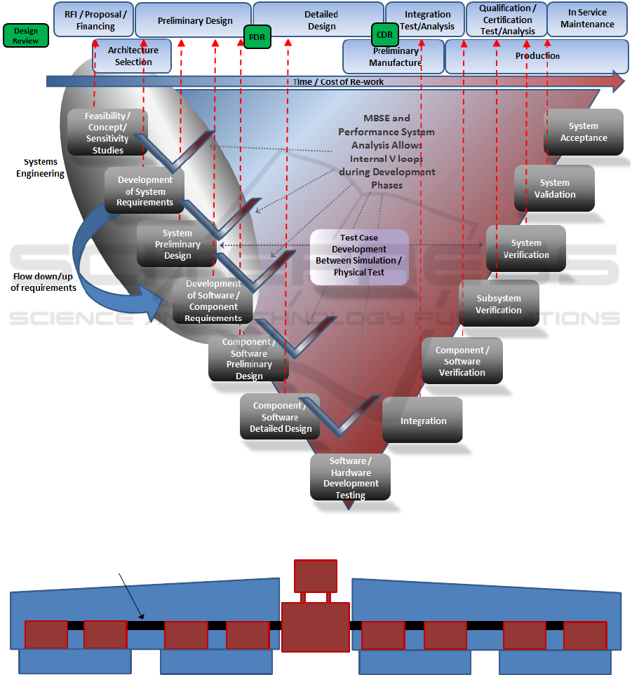
The validation and verification processes based
on modelling and simulation have been further
detailed in Figure 1, whereby iterative cycles of
validation and verification for each stage are
highighted. This process is followed for the
implementation of the functional high lift system.
The work herein presented details the iterative
nature of the preliminary design stage of a product
life cycle. Referring to figure 1, this paper explores
the first level of iteration which enables to derive a
functional framework from customers’ requirements
Hardwick, G. and Panella, I.
Dynamic Modelling of Commercial Aircraft Secondary Flight Control Systems.
DOI: 10.5220/0006418800930101
In Proceedings of the 7th International Conference on Simulation and Modeling Methodologies, Technologies and Applications (SIMULTECH 2017), pages 93-101
ISBN: 978-989-758-265-3
Copyright © 2017 by SCITEPRESS – Science and Technology Publications, Lda. All rights reserved
93
through a process of requirements allocation and
elicitation implemented through modelling and
simulation, specifically through:
• Sensitivity studies
• Trade off analysis
• Test case development
• Decomposition of requirements
The engineering product development schedule
is superimposed with the validation and verification
process to highlight the stages where MBSE can add
value.
In general, model based design emphasises the
use of models through the entire life cycle such as
developing test cases and aiding verification
activities, generating prototype control code,
supporting solving problems, as well as for hardware
in the loop activities and also supporting
certification activities.
Figure 1: Validation and Verification System Design Process.
Figure 2: High Lift architecture.
PDU &
Position
Sensing
Actuator 1 Actuator 1Actuator 2 Actuator 2
Actuator 3
Actuator 3
Actuator 4
Actuator 4
Flap Inboard Surface Flap Inboard Surface Flap Outboard SurfaceFlap Outboard Surface
Controller
Transmission
SIMULTECH 2017 - 7th International Conference on Simulation and Modeling Methodologies, Technologies and Applications
94

2 HIGH LIFT FUNCTIONAL
ARCHITECTURE
The following describes the High Lift Functional
architecture. The architecture shown in Figure 2 is
the result of a previous study presented in Hardwick,
Hanna, and Panella, 2017. It describes a generic
medium sized commercial aircraft flap system,
characterised by a single transmission line and
distributed actuators spaced symmetrically with
respect to the aircraft centreline. This architecture
presents only a flap system and does not include the
slat actuators.
The physical layout includes elements of the
functionalities that a high lift system needs to
present which are:
• Central source Power Drive Unit (PDU) which
provides the power drive actuation to the
system and has position sensing capability;
This interfaces with the secondary flight
controller for control and monitoring functions.
The PDU is dual channel for redundancy.
Hydraulic valves are controlled by the flight
controller and regulate the flow to the
hydraulic motors. The motors drive a
mechanical gearbox that drives the
transmission.
• Transmission shafts connect the PDU to the
actuators on the wing and hence enabling
synchronous movement of both wings.
• Mechanical wing actuation with four rotary
geared actuators (RGA) per wing; These
contain gearboxes which provide mechanical
advantage to the transmission drive torques.
This enables the transmission to drive
aerodynamic loads with large torques.
• The secondary flight control system interfaces
with the PDU, sensors and safety devices
which arrest the system during failure case
scenarios. It also interfaces with the main
aircraft flight controller.
3 MATHEMATICAL MODEL
Herein, the mathematical model of a High Lift
System is described and mapped into a Simulink
model, which is then described.
The model is used to perform a sensitivity study
to support optimal design point for the selection of
the PDU, considering as the key parameter its gear
ratio. A discussion of the model verification is also
presented.
The first step is to define the model
requirements. Requirements enable the definition of
the overall performance requirement for the system,
operational and environmental conditions, as well as
regulatory considerations are needed to ensure
safety. They set the “boundary conditions” for the
systems, which will need to be validated and
verified.
It is important to consider another constraint
when implementing a simulation model. The model
complexity is proportional to run time. Therefore,
the model fidelity needs to be traded with the speed
of simulation that we want to achieve.
Once the requirements are defined, specific
performance descriptions need to be allocated to the
functional blocks, and model outputs are linked to
the systems requirements, such as:
• Flap system deployment times;
• Flap system hydraulic flow rate;
• Dynamic and steady state transmission
loads;
• PDU normal operating velocity.
Dynamic modelling has been achieved through
the application of first order differential equations.
These equations are represented in the form of a
state-space model within the Simulink modelling
environment, which utilises a non-stiff variable step
ordinary differential solver (ODE). The model
contains continuous states but the governing
equations are non-linear and hence the system is a
non-linear time invariant system. State space
modelling is a control systems technique to represent
the dynamic behaviour of a system as reported in
ZadehandDesoer, 1963.
3.1 Model Architecture
The functional architecture is now mapped into the
simulation environment through the application of
mathematical equations capturing the individual
functions’ behaviour, according to mechanical,
hydraulic and electrical physics laws.
Examples of the equations used to create the
blocks are provided in the following sections.
The principle of operation is the following.
Mechanical transmission blocks connect the PDU to
the actuators. The drive to the PDU is generated by
transferring hydraulic power into mechanical using
hydraulic motors.
Figure 3 highlights the system architecture
mapped into a Simulink model. This contains the
following subsystems:
Dynamic Modelling of Commercial Aircraft Secondary Flight Control Systems
95
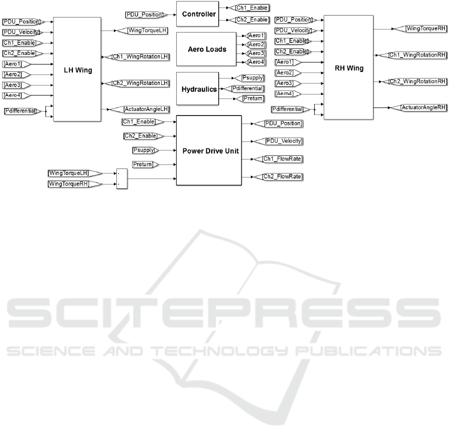
Figure 3: Model architecture of a generic secondary flight control system in Simulink.
• “Controller” is the Secondary flight
controller (which contains I/O to the
aircraft controller);
• “Power Drive Unit” is the Dual channel
power drive unit;
• “LH and RH Wing” are the two mechanical
wings containing the high lift system;
• “Aero Loads and Hydraulics” are the
interface definition of the aerodynamic
loads and hydraulic system.
The PDU and the controller (figure 2) are
translated into the Simulink diagram (figure 3) and
are connected using “GoTo” blocks for example:
• Ch1(2)_Enable – controller to PDU enable
electrical signal.
• PDU_Position – PDU to controller
position
• Aero1(n) – Aerodynamic loads between
the interface and wings
• Psupply – Hydraulic supply pressure
between interface and PDU
3.2 High Lift Transmission
The high lift transmission wing subsystems are
modelled as mechanical blocks that include
component stiffness, inertia, damping, transmission
efficiency and drag. These blocks are defined as
“LH Wing” and RH Wing” in figure 3. A portion of
these blocks have been expanded in figure 4.
Each inertia element contains one dimensional
rotational states (accelerations / velocities). For
example the equation to convert relative
transmission shaft deflection (dx) and velocity (dv)
into a transmission torques is modelled as follows
(where k
trans
and c
trans
are the respective torsional
stiffness and damping of the transmission):
Shaft Torque = k
trans
*dx + c
trans
*dv (1)
Figure 4 provides the Simulink model of the
transmission system including shafts and flap panels
showing the connections between the Simulink
blocks. The shaft torque is multiplied by a
transmission efficiency η
trans
that calculates the
downstream torque for example:
Output Torque = Input Torque*η
trans
(2)
All shaft torques attached to the panel are
summated and then integrated with the aerodynamic
loads into the flap panel dynamic model. This
process is repeated down the transmission line. The
transmission torque and aerodynamic loads are
inputs to the flap panel block.
The net torque acting on the flap panel (T
flap
) is
calculated as follows. The aerodynamic loads (T
aero
)
are converted into the transmission torque reference
frame using the actuator gear ratio (G
act
) and
mechanical efficiency (η
act
). This is summed with
the torque from the transmission shafts (T
trans
) and
drag (T
drag
) is deducted which is described in
equation 3:
T
flap
= (η
act
* T
aero
/ G
act
) + T
trans
-T
drag
(3)
The model contains additional complexities for
example determining the direction of the drag torque
dependant on the direction of rotation.
SIMULTECH 2017 - 7th International Conference on Simulation and Modeling Methodologies, Technologies and Applications
96
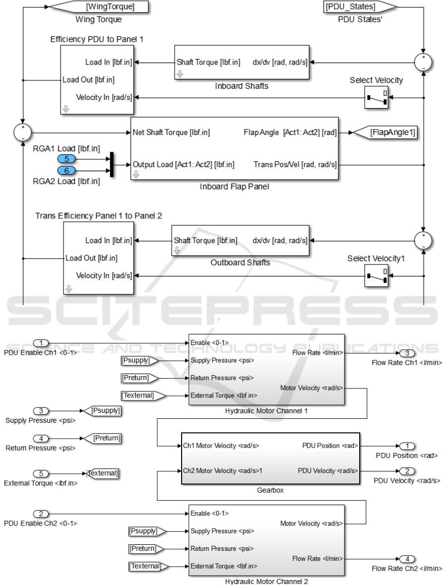
Figure 4: Model of High Lift system in the wing.
Figure 5: Power Drive Unit Model.
Dynamic Modelling of Commercial Aircraft Secondary Flight Control Systems
97
The net torque on the flap panel (T
flap
) is
converted into panel acceleration (A
flap
) by dividing
by the inertia of the panel and transmission
components (I
act
).
A
flap
= (η
act
* T
flap
/ I) (4)
The velocities and displacements are then
determined by integrator blocks.
3.3 Power Drive Unit
The power drive unit model incorporates two
hydraulic channels that contain a constant
displacement motor and control valve to activate the
motor. More complex hydraulic control arrangements
can be used to control the power drive unit more
precisely such as electro hydraulic servo valves.
This block is defined as “Power Drive Unit” in
figure 3 and has been expanded in figure 5.
The PDU enable signal controls both the brake in
the PDU and the control valve. The control valve
dynamics are represented by a first order transfer
function using the time constant T
c
:
Valve Transfer Function = 1/(1 + T
c
.(s)) (5)
Movement of the control valve determines the
pressure drop across (ΔP) the motor. The pressure
drop is converted to a motor torque (T
m
) by
multiplying by the motor displacement (K
mot
) and
incorporating drag (T
drag_m
) and motor efficiency
(η
mot)
as shown by equation 6:
T
m
= ΔP*K
mot
*η
mot
- T
drag_m
(6)
Hydraulic motor acceleration is calculated by
dividing the motor torque by the motor inertia.
Integrating the acceleration provides the angular
velocity of the motor. Both motor speeds are
transferred through a gearbox where the PDU output
shaft position and velocity states are passed to the
wing.
3.4 Secondary Flight System
Controller
The secondary flight control opens the control valve
and releases the system brakes when the position
demand is not equal to the present PDU position.
When the system reaches target position the control
valve is closed and all brakes are engaged.
Multiple brakes are often used in high-lift
systems due to the transmission disconnect failure
scenarios. When activated the brakes prevent
excessive asymmetry between the left and right hand
wing. An actual high-lift controller will typically
have a number of sensors to monitor certain failure
conditions and arrest the system before they become
catastrophic. However, for the purposes of this paper
these are omitted.
3.5 Model Parameters
A list of the model parameters is provided in the
appendix and these are set via the use of Matlab
functions. This allows multiple model parameters to
be run through batches. All parameters used in the
model are arbitrary and do not relate to a particular
aircraft. The model outputs are used to assess the
operating speed of the system and resulting
deployment times. The transmission loads generated
is also analysed.
4 RESULTS
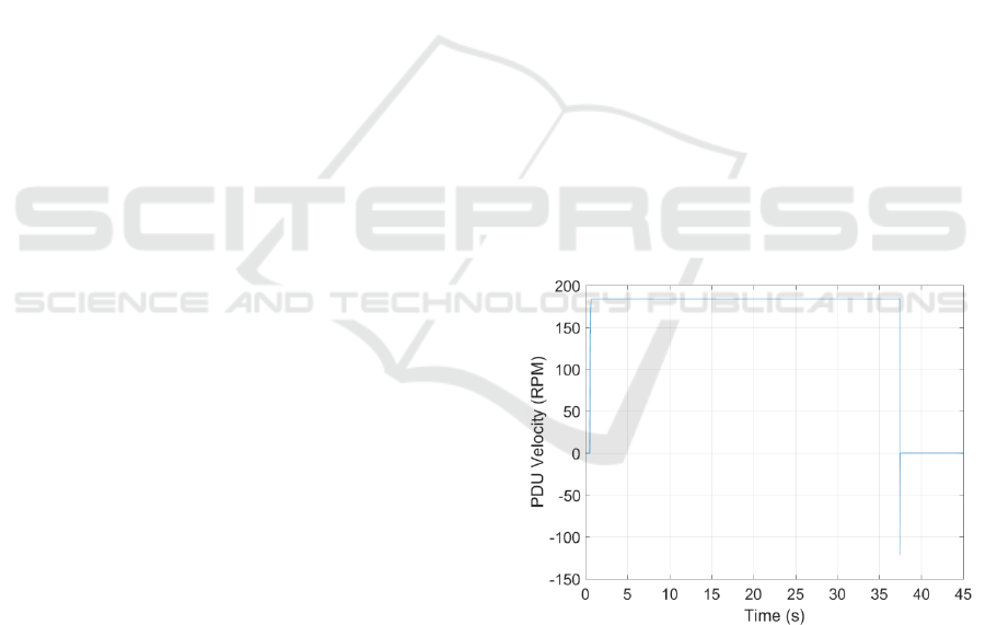
4.1 Time Histories
The basic output from the model is logged in time
histories. Figure 6 highlights the PDU output shaft
velocity during deployment.
Figure 6: Time history of PDU output shaft velocity.
This shows that when the system proceeds at a
normal operating speed of 184 rpm. It takes
approximately 36.9s to fully deploy the system from
the stowed condition.
Both hydraulic motors consume approximately
12.6 l/min flow rate during operation as provided by
figure 7:
SIMULTECH 2017 - 7th International Conference on Simulation and Modeling Methodologies, Technologies and Applications
98
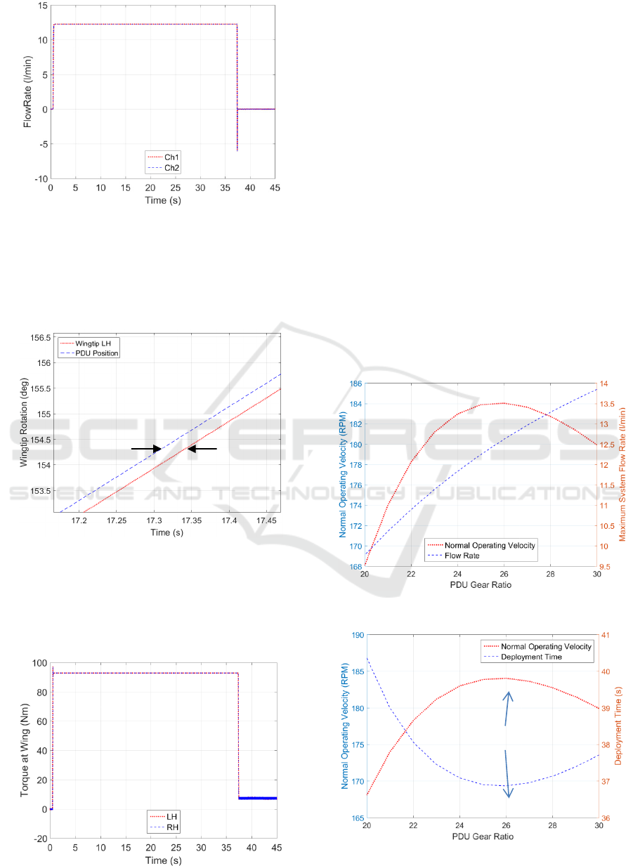
Figure 7: Hydraulic motor flow rate consumption.
The following time history shows the system
position at both the PDU and the wing tips. It can be
seen that the wing tips marginally lag the PDU. The
lag is due to stiffness of the transmission system and
it is the expected systems behaviour.
Figure 8: System Position at the PDU and wing tip
sensors.
Finally the transmission torque from each wing
can be plotted. This shows an initial transient peak
torque at 97Nm reducing to a steady state torque of
93Nm per wing.
Figure 9: Wing torques during deployment.
4.2 Sensitivity Study
The model parameters have been fed into the model
as ranges in order to assess the systems sensitivity.
The example provided shows how the gear ratios of
the PDU gearbox can be modified to achieve various
system requirements such as:
• Minimise running and peak transmission
torques;
• Minimising the hydraulic flow rate
consumption;
• Reducing deployment time.
Figure 10 provides the results from a batch of
simulations where the PDU gear ratio was varied
between 20:1 to 30:1.
The results from the simulations indicate the
optimal gear ratio to be 26:1 which maximises
operating speeds and hence reducing deployment
times. An optimum occurs because of the trade-off
between the mechanical advantage of the PDU and
the drag which increases as function of speed.
Figure 10: Operating velocity and flow rate vs gear ratio.
Figure 11: Normal operating velocity and deployment
time vs gear ratio.
Optimum
Delay in
rotation
between
PDU and
wingtip
Dynamic Modelling of Commercial Aircraft Secondary Flight Control Systems
99
At low gear ratios the PDU has a lower
mechanical advantage and hence the PDU’s torque
capability is lower, which implies lower operating
speeds. At high gear ratios the motor speed is higher
for a given PDU output speed and the speed induced
drag in the motor increases and limits the PDU
speed.
Figure 11 presents the sensitivity analysis of the
variation of the PDU ratio vs. the normal operating
velocity (blue line) and the PDU gear ratio vs. the
deployment time. The optimal gear ratio is the one
defined by the value for which we have operating
velocity and minimum deployment time. In this
example, the optimum PDU gear ratio for this
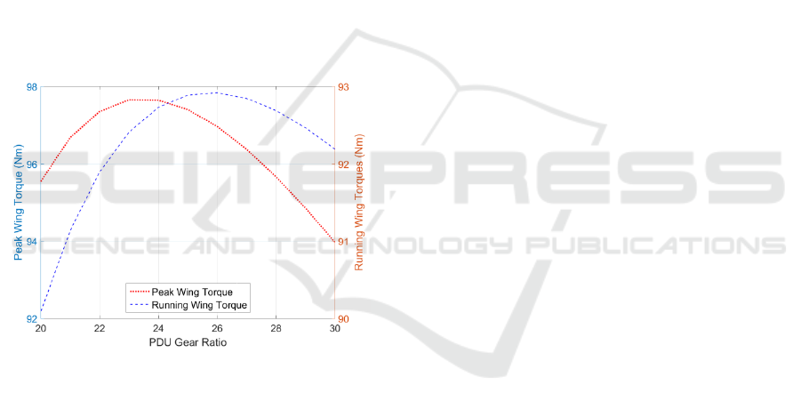
system is 26:1. The transmission torques generated
by the model can be used to as an input into stress
sizing simulations. Figure 12 shows that the running
torques in the transmission are highest at 26:1 due to
the highest operating speeds. The peak transmission
torque has a marginally different trend due to the
dynamic transmission characteristics.
Figure 12: Peak and running torque in the wing
transmission vs gear ratio.
A hydraulic high lift system is typically sized
based upon cold temperature operating and breakout
performance. The reason behind it is that the drag in
the transmission is at the highest while the PDU
capability is the lowest.
5 MODEL VERIFICATION
The mathematical models provided herein have been
verified against physical test data. This has provided
the confidence to use the model outputs to support
the design and development of numerous high lift
aircraft systems.
Model verification has been performed at
numerous stages of the system engineering process
for example at component level (actuator, PDU etc.)
and against full system rig and simulated results.
Excellent model correlation has been achieved at
both individual component and full system level
over a range of environmental temperatures,
aerodynamic loads across multiple programs.
Models have been further utilised in software
and hardware in the loop environments with
suppliers and customers.
Models of secondary flight control systems
developed in the Simulink environment have been
rapid prototyped to support hardware in the loop
simulation.
This has provided the following benefits:
• Development time of software algorithms
significantly improved;
• Control models tested in simulation prior to
integration on the test rigs improve systems’
robustness and easiness of integration.
• Use of the mathematical model as a precise
implementation of the controller and thereby
reducing misinterpretation of formal
requirements.
In recent years there has been a significant shift
in the aerospace industry to move from rig tests to
modelling and simulation environments. Simulations
allow testing of the system in extreme cases that test
rigs may not be able to perform due to:
• Too dangerous/expensive to perform;
• Not possible to perform such as all system
tolerances being maximised/minimised;
• Limitations of the test rigs.
6 CONCLUSIONS
This work has described the modelling process of a
commercial aircraft high-lift transmission and power
drive system. An example model was provided that
was developed in the Simulink modelling
environment and results of a sensitivity analysis
have been provided. Model validation has been
discussed together with the integration of models
into other engineering environments.
This paper provides a generic functional model
and demonstrates the analysis techniques used
within the design and development of high lift
systems that are in-service.
SIMULTECH 2017 - 7th International Conference on Simulation and Modeling Methodologies, Technologies and Applications
100
REFERENCES
Hardwick, G., Hanna, S., Panella, I. 2017. Functional
Modelling of High Lift Systems. NAFEMS World
Congress 2017. NAFEMS, awaiting publication.
Walden, D. 2015. INCOSE Systems Engineering
Handbook 4
th
Ed. INCOSE . WILEY.
SEBoK. 2017. Guide to the Systems Engineering Body of
Knowledge – Validation and verification diagram,
sebokwiki.org.
ARP4754A, 2010, Guidelines for Development of Civil
Aircraft and Systems, SAE International
Zadeh, Desoer, 1963. “Linear System Theory – The State
Space Approach” McGraw Hill, New York
APPENDIX
Table 1: Table of model parameters.
K
hyd
Hydraulic fluid bulk modulus
ρ
hyd
Hydraulic fluid density
I
mot
Hydraulic motor inertia
K
mot
Hydraulic motor displacement
T
s
Control valve time constant
A
valve
Control valve area
C
valve
Coefficient of discharge for control valve
P
PDU
PDU brake disengagement pressure
G
PDU
PDU gearbox ratio
η
mot
Motor efficiency
T
drag_m
Motor drag
k
trans
Transmission torsional stiffness
c
trans
Transmission torsional damping
η
trans
Transmission dynamic efficiency
T
drag
Transmission system drag
I
act
Actuator inertia
T
OBB
Outboard brake response time
P
OBB
Outboard brake disengagement pressure
G
sensor
Gear ratio position sensor
T
aero
Aerodynamic loads at all actuators
G
act
Gear ratios of rotary geared actuators
η
act
Actuator efficiency
Dynamic Modelling of Commercial Aircraft Secondary Flight Control Systems
101
