
Time-energy Optimal Trajectory Planning over a Fixed Path for a
Wheeled Mobile Robot
Werther Alexandre de Oliveira Serralheiro
1
and Newton Maruyama
2
1
Federal Institute of Santa Catarina, Av. XV de Novembro, 61, Ararangu
´
a, Brazil
2
Polytechnic School of the University of S
˜
ao Paulo, Av. Prof. Mello Moraes, 2231, S
˜
ao Paulo, Brazil
Keywords:
Trajectory Planning, Mobile Robot, Convex Optimization.
Abstract:
In this paper a method for time-energy optimal velocity profile planning for a nonholonomic wheeled mobile
robot (WMR) is proposed. Instead of relying on a nonlinear programming algorithm, the method utilizes a
nonlinear change of variables that can transform the nonlinear optimization problem into a convex optimization
problem. The equations are then discretized and later formulated as a second order cone programming that
can be solved by the Matlab CVX toolbox. The formulation of the objective function has two components:
the total energy and the traversal time that is weighted by a parameter named penalty coefficient. With the
use of the penalty coefficient one can easily establish a trade-off between the optimization of total energy and
traversal time. If the penalty coefficient is increased then minimization of time is more prioritized than the
total energy and vice versa. The formulation gives rise to a Pareto optimality condition from which it is not
possible to diminish the traversal time without increasing the total energy and vice versa.
1 INTRODUCTION
The term trajectory planning has been used in
robotics to refer to the problem of determining both
a geometric path and a velocity function for the robot
motion. Although these two sub-problems might be
solved simultaneously, most often, the problem is
solved by first computing a geometric path and then
a velocity profile that satisfies a set of constraints
(LaValle, 2006)
A geometric path can be parameterised by a sin-
gle variable representing the robot travels along the
path. Once the path is reparameterised in this way,
using the robot dynamics, valid velocity profiles can
be determined (Bobrow et al., 1985). Therefore, con-
trol approaches can be used to find a valid velocity
profile that meets certain optimization criteria (Zhao
and Tsiotras, 2013; Pham and Stasse, 2015).
Using the Brobow method, Verscheure et al. (Ver-
scheure et al., 2008; Verscheure et al., 2009) present a
nonlinear change of variables that transform the time
and/or energy optimal trajectory planning problem of
a six DOF robotic manipulator into a convex optimal
control problem to ensure that an optimal solution is
the global one. A Second-Order Cone Programming
– SOCP transformation (Lobo et al., 1998) was also
used in this approach in order to handle with a linear
cost function. Some examples of this approach can be
found in the robotics literature (Ardeshiri et al., 2011;
Reynoso-Mora et al., 2013; Debrouwere et al., 2013;
Zhang et al., 2013).
Lipp and Boyd (Lipp and Boyd, 2014) expand this
approach to find the optimal speed profile for mini-
mum traversal time, given the dynamics of holonomic
vehicles over a fixed path.
Particularly nonholonomic mobile robots bring an
extra challenge for trajectory planning, since they are
characterized by kinematic constraints that are not in-
tegrable and cannot be eliminated from model equa-
tions (Siciliano and Khatib, 2008).
In addition, optimization with non-holonomic
models can not be feasible since there are more dy-
namic equations than optimization variables. Hence,
these equations are no longer constraint on the opti-
mization problem.
The objective and the main contribution of this
work is to present a both time-energy optimization,
expanding from the Lipp and Boyd’s approach, for
an originally nonholonomic wheeled mobile robot
(WMR) model over a fixed path. To this aim, an al-
ternative generalized coordinates system is used to re-
duce the dynamic equations enough to use them in the
optimization, by considering that the fixed path the
robot must traverse is itself a constraint.
Serralheiro, W. and Maruyama, N.
Time-energy Optimal Trajectory Planning over a Fixed Path for a Wheeled Mobile Robot.
DOI: 10.5220/0006398702390246
In Proceedings of the 14th International Conference on Informatics in Control, Automation and Robotics (ICINCO 2017) - Volume 2, pages 239-246
ISBN: Not Available
Copyright © 2017 by SCITEPRESS – Science and Technology Publications, Lda. All rights reserved
239
This paper is organized as follows. In Section
2, a time-energy optimization problem for a class of
wheeled mobile robots is formulated. In Section 3,
the original problem is transformed into a convex op-
timization standard form. The problem is discretized
in Section 4 in order to solve the problem numeri-
cally, and then transformed into a second order cone
programming format which is presented in Section
5. Section 6 presents some numerical results and in
Section 7 some conclusions about this approach are
drawn.
2 PROBLEM STATEMENT
A differential rectangular wheeled mobile robot
(WMR) consists of a rigid frame equipped with two
independent driven wheels. The robot chassis geom-
etry is defined by the width B and the wheels radii
r. Consider p = [x y]
T
the vector representing the
cartesian coordinates of the midpoint P between the
wheels.
Usually, the generalized coordinates of the robot
are given by the vector ξ = [x y θ]
T
, where θ is the
angle between the robot and the inertial coordinate
system. This model has a non-holonomic constraint
since it is underactuated, i.e., the number of the in-
put signals is lower than the size of the generalized
coordinates vector.
Alternatively, consider a vector space where the
time parameterised vectors q : R → R
2
are written in
the form q(t) = [γ(t) θ(t)]
T
, where the monotonically
increasing funtion γ : R → R is the distance traversed
by the robot on the plane from the time 0 to time the
t, and the function θ : R → R is the robot angle as a
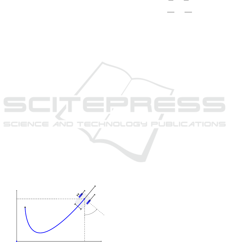
function of the time, as illustrated in Figure 1.
It is easy to prove that the value of the vectors q(t)
do not define the position of the robot on the plane but,
given a start point p
0
, the trajectory of the function q
does.
Y
R
θ(t)
B
r
F
l
(t)
F
r
(t)
F (t)
Y
O
X
O
y(t)
x(t)
P
O
γ(t)
p
0
Figure 1: The WMR dimensions and its pose in two differ-
ent representations ξ and q.
The robot has control inputs u ∈ R
2
, u =
[
u
r
u
l
]
T
, which impose the forces F
r
and F
l
to the
right and left wheels respectively. Given the mass
m and the moment of inertia J of the robot structure,
consider the simplified robot dynamics written as
Ru = M ¨q, (1)
where
R =
K
m
r
K
m
r
K
m
B
2r
−
K
m
B
2r
, (2)
M =
m 0
0 J
, (3)
where K
m
is the DC motor torque constant, and ¨q ∈
R
2
, ¨q = [
¨
γ
¨
θ
]
T
is the acceleration vector.
2.1 Geometric Path Time
Parameterisation
Consider a geometric path as a function s : [0,1] →R
2
that describes the WMR motion, such that
s(τ(t)) = q(t), t ∈ [0,T
f
]. (4)
The function τ : [0,T
f
] → [0,1], named virtual
time, maps the robot motion time in a normalized in-
terval where τ(0) = 0 e τ(T
f
) = 1. This function is de-
fined as monotonically increasing, i.e.,
˙
τ(t) > 0, along
the interval τ = [0,1]. The derivatives of Equation 4
are the robot velocity and acceleration in the configu-
ration space:
˙q(t) = s
0
(τ)
˙
τ(t) (5)
¨q(t) = s
0
(τ)
¨
τ(t)+ s
00
(τ)
˙
τ
2
(t), (6)
where (.)
0
refers to the derivatives in relation with τ.
2.2 Initial Problem Definition
Consider a differential WMR with initial position
p(0) = p
0
and initial configuration q(0) = q
0
mov-
ing along a pre-defined path s(τ(t)) in a time interval
{t ∈ R | t = [0,T
f
]} up to reach a final configuration
q(T
f
) = q
f
.
We want to find a velocity profile ˙q(t), t ∈ [0,T
f
],
such that the robot is driven through the path s in the
minimum traversal time T
f
and energy consumption
E
t
. This problem can be defined as an optimization
problem that can be described as:
ICINCO 2017 - 14th International Conference on Informatics in Control, Automation and Robotics
240

Problem 1. (Minimal time-energy problem)
min.
(u,τ)
: J (t,u) =
Z
T
f
0
ku(t)k
2
2
dt + µ
Z
T
f
0
dt (7)
s.t. : Ru(t) = M ¨q(t) (8)
q(t) = s(τ(t)) (9)
u
min
≤ u(t) ≤ u
max
(10)
˙q
min
≤ ˙q(t) ≤ ˙q
max
(11)
¨q
min
≤ ¨q(t) ≤ ¨q
max
, t ∈ [0,T
f
] (12)
The optimization variables are the virtual time τ
and the input vector u, while the matrices R, M, the
path s and the penalty coefficient µ ∈ R
+
are given
data. The notations (.)
min
and (.)
max
refer respec-
tively to the minimum and maximum values, and the
inequalities given by Equations 10–12 define a poly-
hedra C
t
⊆ R
2x2x2
such that (u(t), ˙q
2
(t), ¨q(t)) ∈ C
t
.
3 CONVEXIFICATION
Using Equation 6 in Equation 1 that defines the WMR
dynamics, yields (Verscheure et al., 2008; Lipp and
Boyd, 2014):
Ru(τ) = M
s
0
(τ)
¨
τ(t)+ s
00
(τ)
˙
τ
2
(t)
. (13)
Two new functions are introduced,
a(τ) =
¨
τ, (14)
b(τ) =
˙
τ
2
. (15)
One can note that
˙
b(τ) = b
0
(τ)
˙
τ, (16)
˙
b(τ) =
d(
˙
τ
2
)
dt
= 2
¨
τ
˙
τ = 2a(τ)
˙
τ, (17)
which results in the following relation
b
0
(τ) = 2a(τ). (18)
The objective function given by Equation 7 can be
redefined, using Equation 15, as
J (τ,u) =
Z
τ(T
f
)
τ(0)
[ku(τ)k
2
2
+ µ]
dτ
˙
τ
=
=
Z
1
0
[ku(τ)k
2
2
+ µ]
p
b(τ)
dτ, (19)
and the nonlinear Problem 1 becomes equivalent to
the following problem:
Problem 2. (Minimal Time-Energy Convex Prob-
lem)
min.
(u,a,b)
: J (τ, u) =
Z
1
0
[ku(τ)k
2
2
+ µ]
p
b(τ)
dτ (20)
s.t. : Ru(τ) = M
s
0
(τ)a(τ) + s
00
(τ)b(τ)
, (21)
b
0
(τ) = 2a(τ), (22)
(u(τ),a(τ),b(τ)) ∈ C
τ
, τ ∈ [0,1], (23)
where
C
τ
= {(u(τ), a(τ),b(τ))|
(u(τ),s
02
(τ)b(τ),s
0
(τ)a(τ) + s
00
(τ)b(τ)) ∈ C
t
}.
The Problem 2 is a convex optimization problem,
since the objective function (Equation 20) is convex,
the equality constraints (Equations 21 and 22) are
afine function of the optimization variables and C
τ
is
a convex set (Boyd and Vandenberghe, 2004).
4 DISCRETE LINEARIZATION
The virtual time τ(t) is an independent variable in
Problem 2. In order to solve the problem numerically
it is necessary to reformulate Equations 20–23 from
continuous time to discrete time. In this context, the
virtual time τ is discretized into N +1 points such that
τ
0
= 0 ≤τ
i
≤ 1 = τ
N
,i = 1, ...,N −1.
On the same way, variables u(τ), a(τ) and b(τ)
have to be discretized into a finite number of vari-
ables: u
i
∈ R
2
; a
i
∈ R , b
i
∈ R; i = 1,.. .,N; and path
s(τ) and its derivatives.
4.1 Discretization of Optimization
Variables
If the time interval between two consecutive points
is small enough, it is possible to consider that vari-
ables a(τ) and u(τ) are constant between two consec-
utive time instants τ
i−1
and τ
i
, i = 1,...,N. Therefore,
both a(τ) and u(τ) are discontinuous in virtual time
τ. These variables are evaluated in the middle point
between two consecutive points as it follows, for all
i = 1,.. .,N,
¯
τ
i
=
τ
i
+ τ
i−1
2
, (24)
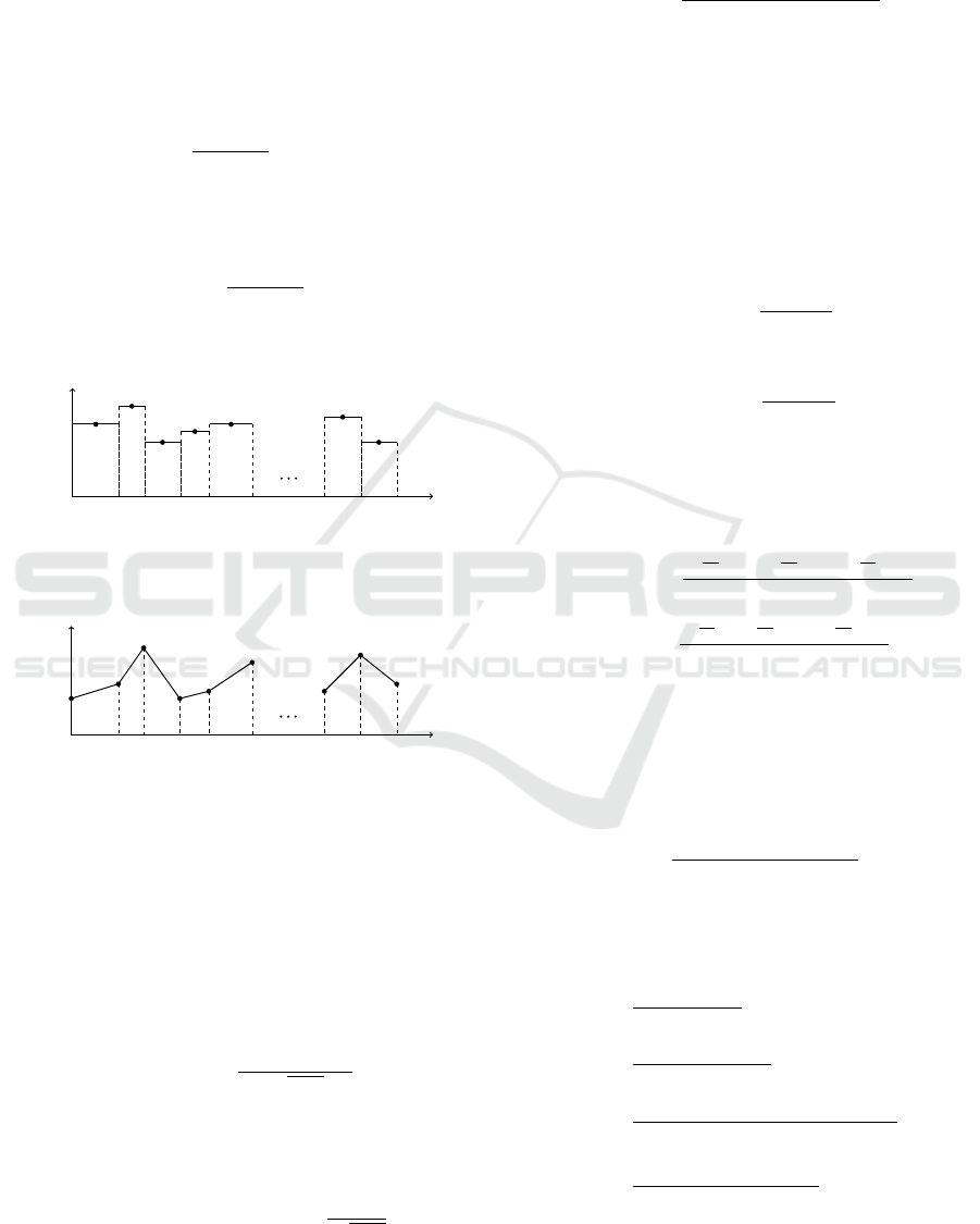
and
a
i
= a(
¯
τ
i
) = a
τ
i
+ τ
i−1
2
, (25)
(See Figure 2) and,
u
i
= u(
¯
τ
i
) = u
τ
i
+ τ
i−1
2
. (26)
Time-energy Optimal Trajectory Planning over a Fixed Path for a Wheeled Mobile Robot
241
On the other hand, b is evaluated in each discrete
point b
i
= b(τ
i
), i = 1,.. .,N. b
0
= b(τ
0
) is defined as
a parameter of the problem.
Since it is assumed that a(τ) is constant and b(τ)
is affine across two consecutive discrete points, b(τ)
might be estimated by a first-order Taylor series ex-
pansion:
b(τ) = b
i−1
+
b
i
−b
i−1
τ
i
−τ
i−1
(τ −τ
i−1
), (27)
for i = 1,...,N, (See Figure 3), while for the middle
point
¯
τ
i
the estimate is given by:
b(
¯
τ
i
) =
b
i
+ b
i−1
2
, (28)
for all i = 1,.. .,N.
a(τ)
τ
τ
1
a
1
τ
0
τ
2
a
2
τ
3
a
3
τ
4
a
4
τ
5
a
5
τ
(N −1)
a
(N −1)
τ
(N −2)
τ
N
a
N
Figure 2: a(τ) is piecewise constant for τ ∈ [0,1] (Adapted
from (Verscheure et al., 2008)).
b(τ)
τ
τ
1
b
0
b
1
τ
2
b
2
τ
0
τ
3
b
3
τ
4
b
4
τ
5
b
5
τ
(N −2)
τ
(N −1)
b
(N −2)
b
(N −1)
τ
N
b
N
Figure 3: b(τ) is piecewise linear for τ ∈ [0,1] (Adapted
from (Verscheure et al., 2008)).
4.2 Discretization of the Optimization
Equations
The objective function of Problem 2 given by Equa-
tion 20 might be rewritten as a sum of definite inte-
grals:
J (τ,u) =
N
∑
i=1
Z
τ
i
τ
i−1
[ku(
¯
τ)k
2
2
+ µ]
p
b(τ)
dτ. (29)
Since u(τ) is constant in each interval it is possible
to write:
J (τ,u) =
N
∑
i=1
(
(ku
i
(
¯
τ)k
2
2
+ µ)
Z
τ
i
τ
i−1
1
p
b(τ)
dτ
)
.
(30)
Using Equation 27 and after some algebraic trans-
formations,
J (τ,u) =
N
∑
i=1
2(ku
i
k
2
2
+ µ)(τ
i
−τ
i−1
)
b
1/2
i
+ b
1/2
i−1
. (31)
The continuous dynamics described by Equation
21 evaluated in the virtual instant time
¯
τ
i
is given by:
Ru(
¯
τ
i
) = M
s
0
(
¯
τ
i
)a(
¯
τ
i
) + s
00
(
¯
τ
i
)b(
¯
τ
i
)
(32)
In order to discretize Equation 32 derivatives of
path s must be estimated. If path s is given in a dis-
crete way, s
i
∈ R
3
, s
i
= s(τ
i
), i = 0,.. .,N the value
of s in the middle point between two consecutive dis-
crete points might be evaluated as
¯s
i
= s(
¯
τ
i
) =
s
i
+ s
i−1
2
, (33)
and the correponding first derivative as
¯s
0
i
= s
0
(
¯
τ
i
) =
s
i
−s
i−1
τ
i
−τ
i−1
, (34)
i = 1,.. .,N.
For the second derivative, an approximation based
on the sixth-order Runge-Kutta symmetric method is
utilized (Lipp and Boyd, 2014):
¯s
00
i
= s
00
(
¯
τ
i
) =
−
5
48
s
i−3
+
13
16
s
i−2
−
17
24
s
i−1
(τ
i
−τ
i−1
)
2
×
×
−
17
24
s
i
+
13
16
s
i+1
−
5
48
s
i+2
(τ
i
−τ
i−1
)
2
. (35)
Since i = 1 ... N, Equation 35 can not be evaluated
at time instants
¯
τ
1
,
¯
τ
2
,
¯
τ
N−1
and
¯
τ
N
. Assuming that the
path s(τ) is linear at its start and at its end, the second
derivatives close to the extremal points might be eval-
uated using the fourth-order Runge-Kutta symmetric
method as
¯s
00
i
=
s
i−2
−s
i−1
−s
i
+ s
i+1
2(τ
i
−τ
i−1
)
2
. (36)
Using this scheme, estimates s
−1
= 2s
0
−s
1
and
s
N+1
= 2s
N
−s
N−1
are obtained.
The complete algorithm is defined recursively as
¯s
00
1
=
s
0
−2s
1
+ s
2
2(τ
1
−τ
0
)
2
, (37)
¯s
00
2
=
s
0
−s
1
−s
2
+ s
3
2(τ
2
−τ
1
)
2
, (38)
¯s
00
(N−1)
=
s
(N−3)
−s
(N−2)
−s
(N−1)
+ s
(N)
2(τ
(N−1)
−τ
(N−2)
)
2
, (39)
¯s
00
N
=
s
(N−2)
−2s
(N−1)
+ s
N
2(τ
N
−τ
(N−1)
)
2
. (40)
Finally, starting from Equations 31 and 32, Prob-
lem 2 is written in discrete-time as:
ICINCO 2017 - 14th International Conference on Informatics in Control, Automation and Robotics
242

Problem 3. (Discrete Minimum Time-Energy Con-
vex Problem)
min.
(u
i
,a
i
,b
i
)
: J(τ,u) =
N
∑
i=1
2(ku
i
k
2
2
+ µ)
√
b
i
+
√
b
i−1
(δτ
i
)
(41)
s.t. : Ru
i
= M
¯s
0
i
a
i
+
¯s
00
i
2
b
i
+
¯s
00
i
2
b
i−1
,
(42)
b
i
−b
i−1
= 2a
i
(δτ
i
) (43)
(u
i
,a
i
,b
i
) ∈ C
¯
τ
, i = 1,.. .,N, (44)
where
C
¯
τ
= {(u
i
,a
i
,b
i
)|
(u(
¯
τ),s
02
(
¯
τ)b(
¯
τ),s
0
(
¯
τ)a(
¯
τ) + s
00
(
¯
τ)b(
¯
τ)) ∈ C
t
},
and δτ
i
= τ
i
−τ
i−1
.
5 FORMULATION AS A SOCP
Though the Problem 3 is a discrete convex optimiza-
tion problem, the objective function in the Equa-
tion 41 is nonlinear. Therefore, four new variables
c
i
,d
i
,e
i
, f
i
∈ R are introduced in Problem 3, where
c
i
> 0, d
i
> 0, e
i
> 0, f
i
> 0, and i = 1, ... ,N, in order
to redefine the objective function as
˜
J (τ,u) =
N
∑
i=1
2(e
i
+ µ f
i
)δτ
i
≥
≥
N
∑
i=1
2(ku
i
k
2
2
+ µ)
√
b
i
+
√
b
i−1
(δτ
i
) =
= J (τ, u), (45)
where the inequalities constraints
1
d
i
≤ f
i
, (46)
u
T
i
u
i
d
i
≤ e
i
, (47)
d
i
≤ c
i
+ c
i−1
, (48)
c
i
≤
p
b
i
, (49)
can be considered as constraints which minimize the
objective function, i.e.,
˜
J ≥ J is an upper constraint
bound of J , it means that minimizing
˜
J ensures that
J is minimal. Moreover,
˜
J is a linear function of the
new optimization variables.
Theorem 1 (Hyperbolic constraints as SOC con-
straints). Given variables w,x,y ∈R with x ≥0, y ≥0
then (Lobo et al., 1998):
w
2
≤ xy ⇐⇒
2w
x −y
2
≤ x + y,
and, more generically, when w ∈ R
n
,
w
T
w ≤ xy ⇐⇒
2w
x −y
2
≤ x + y.
Applying Theorem 1 in the inequalities 46, 47 and
49 it follows
2
d
i
− f
i
2
≤ d
i
+ f
i
(50)
2u
i
e
i
−d
i
2
≤ e
i
+ d
i
(51)
2c
i
b
i
−1
2
≤ b
i
+ 1 (52)
Hence, Problem 3 is equivalent to:
Problem 4. (Discrete Minimal Time-Energy Convex
Problem as a SOCP)
min
(
u
i
a
i
,···, f
i
)
: J (τ,u) =
N
∑
i=1
2(e
i
+ µ f
i
)δτ
i
(53)
s.t. :
2
d
i
− f
i
2
≤ d
i
+ f
i
(54)
2u
i
e
i
−d
i
2
≤ e
i
+ d
i
(55)
2c
i
b
i
−1
2
≤ b
i
+ 1 (56)
d
i
≤ c
i
+ c
i−1
(57)
Ru
i
= M
¯s
0
i
a
i
+
¯s
00
i
2
b
i
+
¯s
00
i
2
b
i−1
,
(58)
b
i
−b
i−1
= 2a
i
(δτ
i
) (59)
(u
i
,a
i
,b
i
) ∈ C
¯
τ
, i = 1,.. .,N, (60)
Solving the Problem 4, the optimal input signal
u
∗
i
and the optimal auxiliary variables (a
∗
,··· , f
∗
) are
found. Thereby, the time t can be re-parametrized by
the rate
δt
i
=
δτ
i
p
b
∗
(τ
i
)
, (61)
as well as the traversal time in seconds and the total
energy consumption in V
2
are calculated by the sums
T
f
=
N
∑
1
δτ
i
p
b
∗
i
, (62)
E
t
=
N
∑
1
ku
∗
i
k
2
2
. (63)
Time-energy Optimal Trajectory Planning over a Fixed Path for a Wheeled Mobile Robot
243
6 RESULTS
In order to validate the proposed method some exper-
imental results are explored in this section.
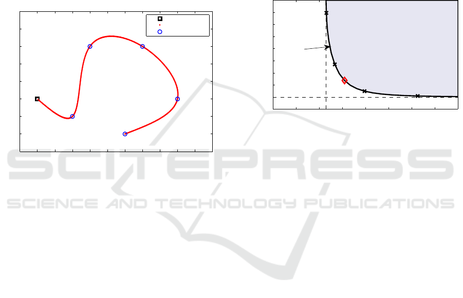
A smoothing spline p is defined with smooth-
ing parameter ρ = 0.99 to reach the following way-
points : p
0
= [
0 0
]
T
, wp
1
= [
2 −1
]
T
, wp
2
=
[
3 −1
]
T
, wp
3
= [
6 −1
]
T
, wp
4
= [
8 −1
]
T
and
wp
5
= [
5 −1
]
T
.
The spline is then divided into N = 500 parts
of equal length, resulting in N + 1 discrete points
p
0
,.. ., p
N
. Figure 4 ilustrates the smoothing spline
p.
−1 0 1 2 3 4 5 6 7 8 9 10
−3
−2
−1
0
1
2
3
4
5
x[m]
y[m]
p
0
p
i
Waypoints
Figure 4: Spline p in the Cartesian plane. The black squared
mark represents the initial point p
0
and the blue circles rep-
resent the waypoints wp
i
, i = 1, ...,5. The red dots are the
discrete points p
i
, i = 1, .. .,N.
Each point p
i
= [
x
i
y
i
]
T
is described by the al-
ternative description in the configuration space s
i
=
[
γ
i
θ
i
]
T
.
The middle points ¯s
i
,(i = 1, ... ,N) are calculated
by Equation 33, the corresponding estimates of the 1st
order derivative ¯s
0
i
by Equation 34 and the 2nd order
derivative ¯s
00
i
by Equation 35 and Equations 36 for the
extremal points of the curve.
A wheeled robot with the following characteris-
tics are considered: width B = 0.4m, inertial mass
m = 10kg, moment of inertia J = 2.833Kg/m
2
, wheel
radius r = 0.1m, DC motor torque constant K
m
= 65 ·
10
−3
Nm/V , nominal input voltage u
max
= −u
min
=
12V .
The robot motion has the following constraints
maximum velocity ˙q
max
= [
2.5m/s 1rad/s
]
T
and
maximum acceleration ¨q
max
= [
2m/s
2
.5rad/s
2
]
T
.
Also the initial value for b
0
= b(τ
0
) = 0. No final
velocity constraint is imposed.
Problem 4 is solved using the algorithm Mosek of
the Matlab CVX toolbox (Grant and Boyd, 2014).
The optimization variables are the left and right
motors input voltage u
i
= [
u
ri
u
li
]
T
, auxiliary vari-
ables a
i
and b
i
, and also auxiliary variables c
i
, d
i
, e
i
e
f
i
, that are defined on Equations 46–49, i = 1, ...,N.
A desktop computer equipped with a 3.60Ghz clock
Intel Core i7-4790, 8GB of RAM running Windows 8
x64 is utilized.
Optimization trials have been performed while
varying the penalty coefficient from µ = 10
−4
up to
µ = 10
4
, with a step size δµ = 10
2.5
. Based on these
trials a graph is designed that represents the traversal
time versus total energy T
f
×E
t
parametrized by the
penalty coefficient µ (See Figure 5).
−10 0 10 20 30 40 50 60 70
−200
0
200
400
600
800
1000
1200
1400
1600
T
f
[s]
E
t
[V
2
]
µ = 10
0
µ = 1 0
1
µ = 1 0
2
µ = 10
3
Possible Region
µ = 40
Pareto
Frontier
Figure 5: Graph of T
f
×E
t
. The shaded region is a possible
set of T
f
×E
t
, limited by the Pareto Front, which converges
asymptotically to the dotted lines. Some values of µ related
to powers of 10 are represented by x marks. µ = 40 is em-
phasized by a red squared mark.
When the penalty coefficient µ decreases towards
zero, µ → 0, the optimization algorithm gradually di-
minishes the importance of the traversal time T
f
while
increasing the importance of the total energy E
t
. As
a consequence the robot velocity diminishes thus in-
creasing the traversal time T
f
. The extreme situation
of µ = 0 ,i.e., only optimization of the total energy
E
t
is of concern, the traversal time is equivalent to
T
f
= 1218s while consuming E
t
= 1.4mV
2
.
On the contrary, if only the optimization of the
traversal time T
f
is important than one can set a very
large penalty coefficient µ → ∞. In this case, the
traversal time is saturated in T
f
= 12.8s and the en-
ergy effort saturated in E
t
= 1704V
2
.
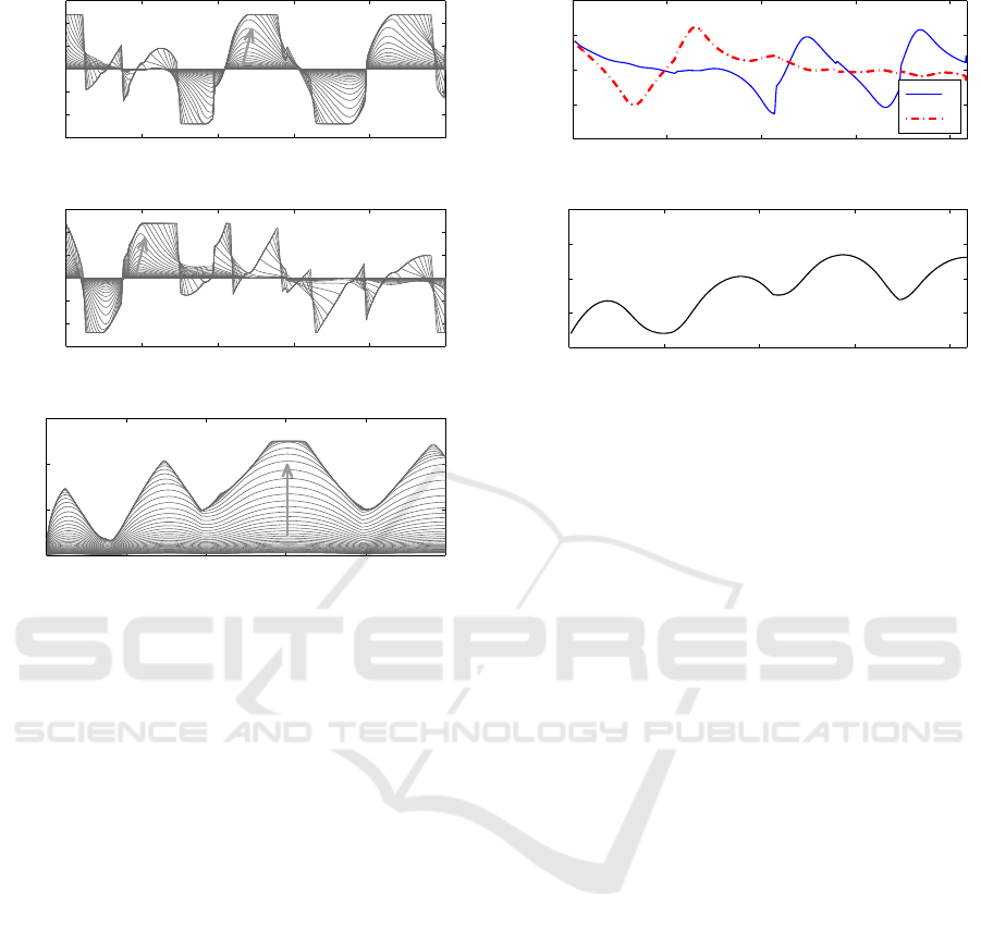
Figure 6 illustrates the series of the optimal input
voltage signals (a) u
∗
r
and (b) u
∗
l
and the optimal ve-
locity profile (c) v
∗
with variation of the coefficient
µ. The arrows shows that the higher the value of µ,
the greater the effort of the motor; consequently, the
greater the linear velocity over the path.
Note some saturation in the input signals (e.g.
on u
∗
r
at i = 250 and on u
∗
l
at i = 120) and the lin-
ear velocity saturation v
max
= 2.5m/s on the inverval
[285 ≤ i ≤ 332].
In Figure 5, it is possible to note a Pareto Knee
ICINCO 2017 - 14th International Conference on Informatics in Control, Automation and Robotics
244
(a)
0 100 200 300 400 500
−15
−10
−5
0
5
10
15
i
u
*
r
[V]
(b)
0 100 200 300 400 500
−15
−10
−5
0
5
10
15
i
u
*
l
[V]
(c)
0 100 200 300 400 500
0
1
2
3
i
v
*
[m/s]
Figure 6: Optimal actuators input voltage signals (a) u
∗
r
, (b)
u
∗
l
and (c) velocity profile v
∗
in function of i. The arrows
indicate the signal trend with the increasing of the penalty
parameter µ.
Point from which it is not possible to diminish the
traversal time T
f
without increasing the total energy
E
f
and vice versa. The red squared mark emphasizes
this point which corresponds to a penalty coefficient
µ = 40. The Figure 7 illustrates the optimal signals for
this particular case, where the traversal time is T
f
=
20.9s and total energy E
t
= 274V
2
.
7 CONCLUSIONS
In this paper a method for time-energy optimal ve-
locity profile planning for a nonholonomic wheeled
mobile robot is proposed.
The main contribution of this work is to consider
an alternative generalized configuration that allows
the use of the previous optimization method (Ver-
scheure et al., 2008; Lipp and Boyd, 2014) for a class
of non-holonomic WMR.
The optimization problem is discretized and later
formulated as a second order cone programming that
can be solved by the algorithm Mosek of the Matlab
CVX toolbox.
The formulation of the objective function has two
(a)
0 5 10 15 20
−10
−5
0
5
10
t[s]
u
*
[V]
u
*
r
u
*
l
(b)
0 5 10 15 20
0
0.5
1
1.5
2
v
*
[m/s]
t[s]
Figure 7: Optimal (a) actuators input voltage signals and (b)
corresponding velocity profile for µ = 40.
components: the total energy E
t
and the traversal time
T
f
that is weighted by a parameter named penalty co-
efficient µ.
As the total energy E
t
is directly related with the
vehicle speed which is inversely related to the traver-
sal time T
f
, only one penalty coefficient µ is neces-
sary to complete specify the trade-off between the to-
tal energy and the traversal time. In this context the
format of the graph of traversal time versus total en-
ergy T
f
×E
t
parametrized by the penalty coefficient µ
(see Figure 5) comes as no surprise.
It is possible to note that the prioritization of the
traversal time is limited by hard constraints like lim-
itation on actuators input voltage, maximum angular
velocity and maximum angular acceleration.
There is a Pareto Knee point from which it is not
possible to diminish the traversal time T
f
without in-
creasing the total energy E
f
and vice versa. A coeffi-
cient µ auto tunning method to find this Pareto Knee
is considered by the authors as a future work.
ACKNOWLEDGEMENTS
This research is being developed under the Inter-
institutional Doctoral Research Program between
Federal Institute of Santa Catarina (IFSC) and
Polytechnic School of the University of S
˜
ao
Paulo (EPUSP), sponsored by the Coordenac¸
˜
ao
de Aperfeic¸oamento de Pessoal de N
´
ıvel Superior
(CAPES). The first author would like to grant the sup-
porting.
Time-energy Optimal Trajectory Planning over a Fixed Path for a Wheeled Mobile Robot
245

REFERENCES
Ardeshiri, T., Norrl
¨
of, M., L
¨
ofberg, J., and Hansson, A.
(2011). Convex Optimization Approach for Time-
Optimal Path Tracking of Robots with Speed Depen-
dent Constraints. In IFAC World Congress, volume 18,
pages 14648–14653. IFAC.
Bobrow, J. E., Dubowsky, S., and Gibson, J. S.
(1985). Time-Optimal Control of Robotic Manip-
ulators Along Specified Paths. The Int. Journal of
Robotics Research, 4:3–17.
Boyd, S. P. and Vandenberghe, L. (2004). Convex Optimiza-
tion. Cambridge University Press.
Debrouwere, F., Van Loock, W., Pipeleers, G., Dinh, Q. T.,
Diehl, M., De Schutter, J., and Swevers, J. (2013).
Time-Optimal Path Following for Robots With Con-
vex - Concave Constraints Using Sequential Con-
vex Programming. IEEE Transactions on Robotics,
29(6):1485–1495.
Grant, M. and Boyd, S. (2014). CVX: Matlab soft-
ware for disciplined convex programming, version
2.1. http://cvxr.com/cvx.
LaValle, S. (2006). Planning Algorithms. Cambridge Uni-
versity Press, New York, NY, USA.
Lipp, T. and Boyd, S. (2014). Minimum-time speed opti-
misation over a fixed path. International Journal of
Control, 87(6):1297–1311.
Lobo, M. S., Vandenberghe, L., Boyd, S., and Lebret, H.
(1998). Applications of second-order cone program-
ming. Linear Algebra and its Applications, 284(1-
3):193–228.
Pham, Q.-C. and Stasse, O. (2015). Time-optimal path pa-
rameterization for redundantly actuated robots: A nu-
merical integration approach. IEEE/ASME Transac-
tions on Mechatronics, 20(6):3257–3263.
Reynoso-Mora, P., Chen, W., and Tomizuka, M. (2013).
On the time-optimal trajectory planning and control of
robotic manipulators along predefined paths. Amer-
ican Control Conference (ACC), 2013, (November
2016):371–377.
Siciliano, B. and Khatib, O., editors (2008). Springer Hand-
book of Robotics. Springer Berlin Heidelberg, Berlin,
Heidelberg.
Verscheure, D., Demeulenaere, B., Swevers, J., De Schut-
ter, J., and Diehl, M. (2008). Time-energy optimal
path tracking for robots: a numerically efficient opti-
mization approach. In IEEE International Workshop
on Advanced Motion Control, pages 727–732, Trento.
IEEE.
Verscheure, D., Demeulenaere, B., Swevers, J., De Schutter,
J., and Diehl, M. (2009). Time-optimal path tracking
for robots: A convex optimization approach. IEEE
Transactions on Automatic Control, 54(10):2318–
2327.
Zhang, Q., Li, S.-R., and Gao, X.-S. (2013). Practical
smooth minimum time trajectory planning for path
following robotic manipulators. 2013 American Con-
trol Conference, pages 2778–2783.
Zhao, Y. and Tsiotras, P. (2013). Speed Profile Optimiza-
tion for Optimal Path Tracking. In American Control
Conference (ACC), pages 1171 – 1176.
ICINCO 2017 - 14th International Conference on Informatics in Control, Automation and Robotics
246
