A Hybrid Prediction Model Integrating Fuzzy Cognitive Maps with

Support Vector Machines

Panayiotis Christodoulou, Andreas Christoforou and Andreas S. Andreou

Department of Electrical Engineering / Computer Engineering and Informatics, Cyprus University of Technology,

31 Archbishop Kyprianos Street, Limassol, Cyprus

Keywords: Fuzzy Cognitive Maps, Prediction, Machine Learning, Support Vector Machine, Weighted k-NN, Linear

Discrimination, Classification Tree.

Abstract: This paper introduces a new hybrid prediction model combining Fuzzy Cognitive Maps (FCM) and Support

Vector Machines (SVM) to increase accuracy. The proposed model first uses the FCM part to discover

correlation patterns and interrelationships that exist between data variables and form a single latent variable.

It then feeds this variable to the SVM part to improve prediction capabilities. The efficacy of the hybrid

model is demonstrated through its application on two different problem domains. The experimental results

show that the proposed model is better than the traditional SVM model and also outperforms other widely

used supervised machine-learning techniques like Weighted k-NN, Linear Discrimination Analysis and

Classification Trees.

1 INTRODUCTION

Prediction is a vital issue that applies in every

scientific discipline, while at the same time it is also

considered a problem involving multiple and usually

conflicting factors; therefore, the prediction process

may be considered as highly complex exhibiting

high levels of uncertainty. This problem is

particularly challenging leading to the development

of a large number of approaches and tools to provide

accurate results. Substantial effort has been recorded

in the research community focusing mainly on two

major aspects of the prediction models: On one hand

accuracy is the most important aspect of prediction

and its value characterizes the model’s performance;

on the other hand, the timeliness of delivering

accurate predictions is equally important.

Aiming to tackle the aforementioned challenges

this paper introduces a new hybrid prediction model

called SVM-FCM that exploits the advantages

offered by Fuzzy Cognitive Maps (FCMs) coupled

with the prediction abilities of Support Vector

Machines (SVM) to produce a more accurate model

that is able to provide results timely.

FCMs are essentially graph-based cognitive

models that work and behave like recurrent Artificial

Neural Networks (ANNs) with some differences.

They can model any real-world problem by

capturing its dynamics and represent cognitive

knowledge in the states of its nodes. The nodes,

known also as concepts, influence each other in a

finite iterative cycle, which, eventually, and under

certain conditions, is terminated at equilibrium or

bounded oscillating state delivering the final output

of the model. Such kinds of models have extensively

been used with success in a wide range of

applications and disciplines exhibiting an

exponential growth in the last ten years

(Papageorgiou, 2013, Papageorgiou and Salmeron

2013). FCMs exhibit various advantageous features

over other models, such as strong knowledge

representation, uncertainty handling, dynamic

behavior and ease of understanding and use, which

make them ideal for problem simulation, analysis

and tendency prediction in various domains. Among

other applications, a number of FCM models have

been proposed in multivariate time series prediction,

which presents significant similarities with real time

prediction.

In this research work we aim to benefit from the

FCM capabilities so as to capture the dynamics of a

complex non-linear problem and deliver an output in

the simplest possible form. This output will then be

integrated with the SVM part of the model to assist

554

Christodoulou, P., Christoforou, A. and Andreou, A.

A Hybrid Prediction Model Integrating Fuzzy Cognitive Maps with Support Vector Machines.

DOI: 10.5220/0006329405540564

In Proceedings of the 19th International Conference on Enterprise Information Systems (ICEIS 2017) - Volume 1, pages 554-564

ISBN: 978-989-758-247-9

in improving its accuracy. This study was motivated

by the following research questions:

RQ1 - Is a Fuzzy Cognitive Map (FCM) able to

model a multivariable environment and handle its

complexity?

RQ2 – How can a FCM model transform a

multivariable environment to a single collective

output that will increase the accuracy of a SVM

model?

For finding answers to the aforementioned questions

this paper contributes the following: (a)

Development of a FCM model tailored to the

problem in hand and execution of this model using

various training datasets to discover hidden

correlations between the input data; (b) Integration

of the FCM model with a SVM model that takes into

consideration the latent FCM variable formed and

use it to increase the hybrid system’s overall

prediction accuracy; and (c) Experimentation using

two well-known datasets, occupancy and diabetes,

and comparison with other similar approaches.

The rest of the paper is structured as follows:

Section 2 reviews related work on the topic, while

section 3 describes an overview of the proposed

approach and discusses the technical background.

Section 4 presents the experimental part, evaluates

the results and discusses the comparison of the

model with other baseline approaches. Finally,

section 5 concludes the paper and presents future

research steps.

2 RELATED WORK

This section starts by briefly presenting work using

the datasets utilised in this paper and then focuses on

the use of the underlying models in prediction

problems.

The accuracy of predictions that depends on

occupancy using various data attributes (light,

temperature, humidity and CO2) was first presented

in (Candanedo and Feldheim, 2016). That paper uses

three datasets, one for training the models and two

for testing them. A number of training models such

us the Linear Discriminator Analysis (LDA),

Regressions Trees and Random Forests were used

for training and testing purposes. The best

accuracies obtained from the several experiments

range from 95% to 99%. Results showed that the

impact of accuracy on each experiment depends on

the classification model and the number of features

selected each time. Taking into consideration all of

the features the best accuracy was resulted using the

LDA model for both test datasets.

The paper described in Smith et al. (1988) is

using a neural network to predict the diabetes

mellitus for a high risk population in India. It was

one of the first algorithms used on health

forecasting. The proposed methodology was

compared with other models achieving a high

accuracy of 76%.

Ster et al. (1996) test a number of classification

systems on various medical datasets (Diabetes,

Breast Cancer and Hepatitis) in order to obtain

accurate results when using a number of different

methods. In terms of classification accuracy in most

of the datasets the neural networks approaches

outperform other methods such as Linear

Discrimination Analysis (LDA), K-nearest neighbor,

Decision Trees and Naïve Bayes.

In Papageorgiou et al. (2016), a new hybrid

approach based on FCM and ANN is presented for

dealing with time series prediction. The proposed

model was applied and tested in predicting water

demand on the island of Skiathos. The methodology

presented increases prediction accuracy of ANN by

using concepts from FCMs as input data.

Authors in (Papageorgiou and Poczeta, 2015)

conducted a multivariate analysis and forecast of the

electricity consumption with a 15-minute sampling

rate using three different FCM learning approaches:

multi-step gradient method, RCGA and SOGA.

These approaches found to be more suitable for the

electricity consumption prediction rather than

popular artificial intelligent methods of ANNs and

ANFIS.

Shin et al. (2005) investigate the application of a

SVM model to a bankruptcy prediction problem.

Even though it is known from previous studies that

the back-propagation neural network (BPN)

produces accurate results when dealing with pattern

recognition tasks, it faces limitations on constructing

an appropriate model for real-time predictions.

The proposed classification model based on SVM

captures the characteristics of a feature space and is

able to find optimal solutions using small sets of

data. The suggested approach performs better than

the BPN in terms of accuracy and performance when

the training size decreases.

The paper presented in (Mohandes et al., 2004)

introduces a SVM model on a wind speed prediction

problem. The performance of the proposed

methodology was compared with a multilayer neural

network (MLP). The dataset used for experimental

purposes was recorded in Asia and the results based

on the RMSE error between the actual and predicted

data showed that the SVM approach outperforms the

MLP model.

A Hybrid Prediction Model Integrating Fuzzy Cognitive Maps with Support Vector Machines

555

Cortez and Morais (2007) explore different

machine learning techniques in order to predict the

burnt area of forests. Two models, SVM and

Random Forests, were tested offline on a real-world

dataset collected from a region in Portugal. On each

experiment the two models make use of various

features and their accuracies are computed. The best

approach used the SVM algorithm with all

meteorological data as input and was able to predict

the burnt area of small fires which happen more

frequently. A drawback of this approach is that it

cannot predict with high accuracy the burnt area of

larger fires; this is feasible only by adding additional

information to the model.

Finally, a similar approach is followed by

Papageorgiou et al. (2006) that presents a Fuzzy

Cognitive Map (FCM) trained using a Nonlinear

Hebbian Algorithm combined with Support Vector

Machines (SVMs) in order to address the tumor

malignancy classification problem by making use of

histopathological characteristics. The hybrid model

achieves a classification accuracy of 89.13% for

high grade tumors and 85.54% for low grade tumors

and outperforms on overall accuracy the k-nearest

neighbor, linear and quadratic classifiers.

Nevertheless, this methodology uses a SVM

approach to classify the data and not to train the

model.

The relevant literature on prediction, as well as

on the use of SVM and FCM models is vast. Our

intention was to show indicative examples of

problems that these models may tackle, their

prediction strengths and abilities, and the diversity

of the application domains that may be benefitted by

them, so as to provide a form of justification for

their selection as the constituents of our hybrid

model.

3 OVERVIEW OF APPROACH

This section presents the approach for developing a

FCM model to discover hidden correlations that may

exist in the training data and subsequently

integrating these correlations with a SVM model

aiming to increase its accuracy.

3.1 Fuzzy Cognitive Maps

Fuzzy Cognitive Maps (FCMs) are tools which

inherit elements from the theory of fuzzy logic and

neural networks (Kosko, 1992, Kosko, 1993). The

FCM approach was firstly proposed by Kosko as an

extension of Cognitive Maps (Kosko, 1986) and was

used for planning and as decision support tools in

various scientific fields, such as social and political

developments, urban planning, agriculture,

information and communication technology,

software engineering and others (Kosko, 2010,

Kandasamy and Smarandache, 2003). Their simple

nature and ease of understanding led them to a wide

range of applications. Essentially, a FCM is a

digraph with nodes representing concepts in the

domain of a problem and directed edges describing

the causal relationships between those concepts. A

positively weighted directed edge between two

concepts indicates a strong positive correlation

between the causing and the influenced concept.

Inversely a negatively weighted directed edge

indicates the existence of a negative causal

relationship. Two conceptual nodes without a direct

link are, obviously, independent. Each concept node

keeps a numerical value as an activation level in the

range [0, 1], and indicates the strength of its

presence in the problem under study. The number of

nodes and the number of their causal relationships,

denote the degree of complexity of the map.

Additional complexity appears with the presence of

cycles between nodes, that is, paths starting and

ending on the same nodes.

As originally proposed, a FCM is constructed

with the aid of a group of experts who, based on

their knowledge and expertise, identify the nodes

that are relevant to the problem under study and

define the activation levels of the concepts, as well

as the weights of the causal relations between them.

The model is then executed on a series of discrete

steps (Kosko, 1986) during which the activation

levels of the participating concepts are iteratively

calculated for a number of repetitions and at the end

the model can either reach an equilibrium state at a

fixed point, with the activation levels reaching stable

numerical values, or exhibit a limit cycle behavior,

with the activation levels falling in a loop of

numerical values under a specific time-period, or

present a chaotic behavior, with the activation levels

reaching a variety of numerical values in a random

way. In the former two cases of value stabilization

inference is possible.

The activation level of a node denotes its

presence in the conceptual domain and is calculated

taking into account the activation levels of the nodes

from which it is fed, as well as its own current

activation. The activation level of each node is

calculated using the following equation:

1t t t

i ij i j

x f w x x















(1)

ICEIS 2017 - 19th International Conference on Enterprise Information Systems

556

where f is a threshold function that keeps an

activation level value in the desired interval and it

can be chosen from a number of available functions

(Bueno and Salmeron, 2009) based on the nature of

the model and the problem in hand. The sigmoid

function is the most widely used function and

squashes the value of the function in the interval [0,

1]:

 









(2)

In this work the FCM model is used to discover the

latent variable FCM

OUT

that will be later used as

input to the SVM model.

3.2 Support Vector Machines (SVM)

SVM is a supervised machine learning approach that

analyzes data for classification. It constructs a model

and assigns instances in different categories. The

instances are represented as points in the feature

space and they are divided by a hyperplane (Cortes

and Vapnik, 1995). When new data is available it is

mapped into the space and the model predicts the

specific category it belongs to depending on the side

of the hyperplane it falls on.

The aim of a SVM model is to find and select the

best hyperplanes to separate the data. This paper

utilises a Linear SVM algorithm that consists of the

following steps:

Step 1: Hyperplanes

Given a hyperplane H

that separates D and satisfies:

0 w x b  

(3)

where

is a weight and

is a threshold.

Select two other hyperplanes H

and H

that also

separate the data with equations:

w x b



  

(4)

w x b



   

(5)

where δ is a variable, so that the distance of H

from

and H

is equal.

Each vector

can belong to a class when:

w x b  

(6)

w x b   

(7)

Combining both equations above we get a unique

constraint where there are no points between the two

hyperplanes:

) 1(

y w x b  

for all

1 in

(8)

where x

is the i

training sample and y

is the correct

output.

Step 2: Margin

The hyperplane that has the largest margin between

the two classes is used as the best choice to classify

the data.

The margin is calculated using the formula below:



 

(9)

To calculate the optimal hyperplane the SVM finds

the couple (w, b) for which

w 

is minimized

subject to:

) 1(

y w x b  

1, ,in

(10)

where x

is the i

training sample and y

is the correct

output.

Step 3: Classification

The algorithm is trained to find the best hyperplane

using the previous steps; it then uses the test data to

predict the specific class each sample belongs to.

3.3 SVM-FCM Model

The FCM plays a central role to this model. We aim

at capturing the tendency of the input dataset and

deliver a linear output “aligned” with the real

predicted value.

3.3.1 FCM Construction

A semi-automated learning method for the FCM

construction is proposed which is based on the

correlations between the input variables calculated

using historical data in combination with literature

review on the topic and domain experts consultation.

The proposed approach follows a stepwise process

described in details below:

Step 1: Pre-processing

At this step the historical data is fed using a pre-

processing procedure during which a linear

normalization is performed that transforms the input

data set values in the range [0, 1].

min

max min

' , 1..

x i n







(11)

Step 2: Correlation Matrix Calculation

A strong indication of the dependence between the

input variables is given by calculating their

correlation and associated p-values.

A Hybrid Prediction Model Integrating Fuzzy Cognitive Maps with Support Vector Machines

557

Step 3: Literature Review & Expert Consultation

The connections between the concepts in a FCM

represent the one-way causality from one to another.

By default correlation is not causality, i.e. we cannot

safely argue about the source and destination of

causalities between two correlated nodes; thus, we

need to examine this issue further. We resort to

using domain experts and/or knowledge extracted

from the relevant literature to accept or discard

possible causalities as these are extracted from the

correlation matrix and then decide upon the direction

of each causality. In addition, we make some valid

assumptions that come logically and effortlessly

regarding variables that depend on time such as day,

week etc. which cannot be influenced by any other

variable.

Step 4: FCM Analysis & Calibration

A significant factor that greatly affects FCM

performance is the selection of the activation level

equation, as well as the selection of the threshold

function. The criteria for this decision may be

attributed to the map’s balance based on negative

and positive cycles created, the input and output data

format, etc.(Andreou et al., 2005).

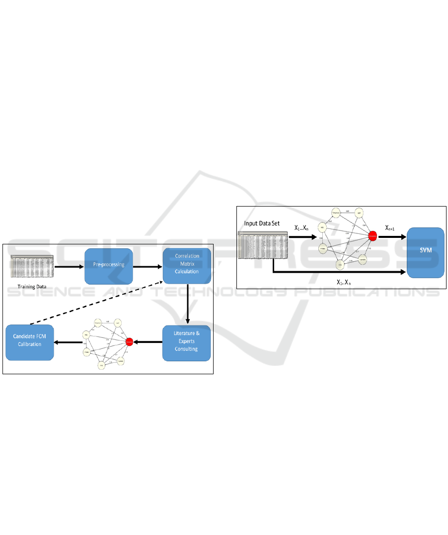
Figure 1: FCM model construction.

The performance evaluation of a FCM can be

made by assessing the success rate of the model over

training data, aiming to reach the maximum possible

level. Based on the type of real reference values we

can define the form of the model’s output, FCM

OUT

For example, if the reference values’ class is binary,

we may seek for a threshold that could separate

FCM

OUT

values in such a way so as to deliver the

maximum matching between the predicted class

FCMout

, and the actual x

values as follows:

 

max | | , 1.. ,

1,if ,

x FCMout i n

FCMout FCMout threshold

FCMout otherwise

 





(12)

In the case of a scalar reference value type a

regression analysis can be applied using the FCM

OUT

values as the dependent variable x and the reference

values as the explanatory variable y:

y ax





(13)

Steps 2, 3 and 4 of the FCM analysis and

calibration process may be repeated leading to the

construction of the final FCM model as depicted

graphically in Figure 1.

The construction of the hybrid model (see

Figure 2) comprises two sequential steps: The

creation and execution of the FCM model that

utilises the available dataset to discover the latent

variable FCM

OUT

; the use of FCM

OUT

as input, along

with the rest inputs sourced by the same dataset, by

the SVM model and generation of predictions.

Figure 2: SVM-FCM model.

4 EVALUATION

Aiming to evaluate the performance of the proposed

approach, we applied the SVM-FCM model on two

different datasets, the first consisting of data samples

describing an occupancy problem and the second

one comprises real-world samples for the diabetes

disease. Both datasets are available in (Asuncion and

Newman, 2007). For comparison purposes we also

implemented various baseline approaches described

briefly below, which were executed over the same

datasets to assess the accuracy of the proposed

model.

4.1 Comparative Baseline Approaches

The hybrid model was compared in terms of

accuracy against the classic Linear SVM model and

the following baseline algorithms which are the most

ICEIS 2017 - 19th International Conference on Enterprise Information Systems

558

widely used in literature for classification prediction

purposes:

4.1.1 Weighted k-NN

The k-NN is one of the most well-known approaches

used for classification. This algorithm first finds a

number of k nearest neighbours for each instance by

measuring a distance using various metrics. Then it

uses that metric to classify each instance taking into

consideration the majority label of its nearest

neighbours (Gou et al., 2012). This paper uses a

variation of the traditional k-NN approach called

Weighted k-NN which provides a higher weight to

closer neighbours and better accuracy than the

normal k-NN.

4.1.2 Linear Discrimination Analysis

Linear discrimination analysis (LDA) is an approach

used in statistics and machine learning in order to

find a linear combination of features that separates

two or more classes of instances (McLachlan, 2004).

LDA follows three steps:

Step 1:

LDA separates the instances x

given in the dataset D

into various groups based on the value of their class.

Then it computes the μ value of each dataset and the

global μ value of the entire dataset and subtracts

those values from the original ones.

Step 2:

The covariance matrix of each group is found and

then the pool covariance matrix is calculated using

the formula below:

( , )

C p c r s





(14)

where c

is the covariance matrix of group i, (r,s) is

each entry in the matrix and p is the prior probability

computed by:



(15)

where n

defines the total samples of each group and

N the total samples of the dataset.

Step 3:

The inverse matrix C

-1

is calculated and used in the

discrimination function which aims to assign each

instance to a class as follows:

ln( )

i i i i

f C x C p



  



  

(16)

4.1.3 Classification Tree

Classification tree (CT) learning is a commonly used

method in machine learning that constructs a tree-

like model aiming to predict the class of an instance

based on the input of a training dataset (Loh, 2011).

In a classification tree model the leaves present the

class of an instance and the branches describe the set

of features that lead to a leaf (class); therefore,

following the decisions from the beginning of the

decision tree down to the leaves the classes are

predicted.

4.2 Parameters

This section provides a brief summary of the main

parameters used for executing the baseline

algorithms and the proposed model.

First of all, a k-fold (k=5) cross validation was

performed on all training models.

The Weighted k-NN model takes into

consideration the 10 closest neighbours (k=10), uses

the Euclidean distance metric to measure the

similarity between instances and the weight is

measured using the formula below:

𝑑𝑖𝑠𝑡𝑎𝑛𝑐𝑒

(17)

The LDA model uses the Baye’s Theorem to

calculate probabilities; then the classifier is

constructed based on a linear combination of the

dataset’s input where the delta threshold is set to 0

and the gamma regularization parameter to 1.

The CT model uses a continuous type of cut at

each node in the tree and the Gini’s diversity index

(gdi) criterion for choosing a split.

The SVM model uses a linear kernel function to

calculate the classification score of instances and a

gradient descent for minimizing the objective

function.

4.3 Accuracy

The accuracy metric used for computing the

accuracy and evaluating the methods on both test

datasets was the following:

Accuracy

A B C D





  

(18)

where the A, B, C and D variables are defined in the

confusion matrix shown in Table 1.

A Hybrid Prediction Model Integrating Fuzzy Cognitive Maps with Support Vector Machines

559

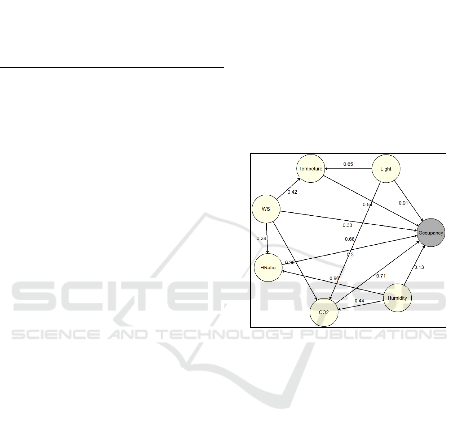
Table 1: Confusion Matrix.

Approach

Predicted

Value=1

Predicted

Value=0

Reference

Value=1

Reference

Value=0

4.4 Occupancy Dataset

The occupancy datasets used in this paper were

presented in Candanedo and Feldheim (2016). The

data samples were collected from sensors installed in

an office room, while a digital camera was used to

find out the occupancy of the room.

Each dataset has the following attributes: Date

and time in the format of year-month-day

hour:minute:second, Temperature measured in

Celsius (T), Relative Humidity in % (φ), Light

measured in Lux (L), CO2 in ppm (CO2) and the

Humidity Ratio (W) that is calculated by dividing

the temperature and relative humidity. Occupancy

(O) is either 0 for not occupied or 1 for occupied

status. The utilization of date-time stamp in all

datasets has been expressed by extracting two more

variables: Number of seconds since midnight (SSM)

and week status (WS) that is either 0 for weekend or

1 for weekday. The training dataset consists of 8143

records with 7 attributes (6 attributes from the

original dataset plus the attribute resulted in by the

FCM) and the two test datasets consist of 2665 and

9572 records respectively with 6 attributes (5

attributes from the original datasets plus the FCM

attribute).

The aforementioned datasets were used to train

and test the proposed model and the baseline

algorithms for comparison purposes. The datasets

used with the proposed approach also include the

variable discovered by the Fuzzy Cognitive Map.

The occupancy attribute of the test datasets was used

for evaluating and comparing the proposed approach

against the baseline methods.

4.4.1 Modelling

Following the model construction procedure

described above, we proceeded and utilized the

available dataset to construct and evaluate the

proposed model.

Firstly, a linear normalization was applied to the

datasets, as a result of which values in both the

training and the test dataset were transformed in the

range [0, 1]. Subsequently, the correlation matrix

was calculated and it is presented in Table 2 with p-

values appearing in parentheses.

Based on the findings extracted from the

correlation and associate p-values we identified pairs

with high linear significant relationships. In

addition, to support this procedure, we defined and

set some rules towards causality identification. We

eliminated the SSM variable since its values do not

have a continuous and linear relationship with the

Occupancy variable. We also inferred that the time

depended variable WS cannot be influenced by any

other variable. Finally, we consulted the relevant

literature, where and when necessary, to identify the

value and the direction of an influence.

Figure 3: Final FCM model for the occupancy dataset.

The FCM model that emerged from this process

is shown in Figure 3 with its associated edge-weight

values. It is obvious that the constructed FCM is a

fully positive map consisting exclusively of positive

cycles. This evidence guided us to the selection of

the update and threshold functions in such a way so

as to increase the model’s sensitivity to uncertainty

and to quantization of the final value.

The sigmoid function with λ=1, was chosen as

the threshold function and the update function is

described in equation (19) below (Iakovidis and

Papageorgiou 2011):

(2 1) (2 1)

t t t

i ij i j

x f w x x







   







(19)

We performed a number of executions on the

FCM model to check its accuracy performance. For

each execution we ran 50 iterations and managed to

reach equilibrium in all executions and to deliver a

stable value for FCM

OUT

. The binary type of the

ICEIS 2017 - 19th International Conference on Enterprise Information Systems

560

Table 2: Correlation Matrix and p-values in parentheses for the occupancy dataset.

SSM

CO2

0.00

-0.01

(0.33)

0.42

(0.00)

0.11

(0.00)

0.28

(0.00)

0.39

(0.00)

0.24

(0.00)

0.38

(0.00)

SSM

-0.01

(0.33)

0.00

0.26

(0.00)

0.02

(0.00)

0.09

(0.00)

0.21

(0.00)

0.10

(0.00)

0.08

(0.00)

0.42

(0.00)

0.26

(0.00)

0.00

-0.14

(0.13)

0.65

(0.00)

0.56

(0.00)

0.15

(0.00)

0.54

(0.00)

0.11

(0.00)

0.02

(0.13)

-0.14

(0.00)

0.00

0.04

(0.00)

0.44

(0.00)

0.96

(0.00)

0.13

(0.00)

0.28

(0.00)

0.09

(0.00)

0.65

(0.00)

0.04

(0.00)

0.00

0.66

(0.00)

0.23

(0.00)

0.91

(0.00)

CO2

0.39

(0.00)

0.21

(0.00)

0.56

(0.00)

0.44

(0.00)

0.66

(0.00)

0.00

0.63

(0.00)

0.71

(0.00)

0.24

(0.00)

0.10

0.15

(0.00)

0.96

(0.00)

0.23

(0.00)

0.63

(0.00)

0.00

0.30

(0.00)

0.38

(0.00)

0.08

(0.00)

0.54

(0.00)

0.13

(0.00)

0.91

(0.00)

0.71

(0.00)

0.30

(0.00)

0.00

reference occupancy value (0 or 1) allowed us to use

a threshold value of 0.27 achieving 98.8% accuracy

on the training input data.

After the finalization of the FCM model the

hybrid FCM-SVM model was executed on the two

test datasets.

4.4.2 Execution Results and Comparison

Table 3 presents the accuracy of the predictions for

the baseline approaches, as well the accuracy of the

proposed hybrid SVM-FCM model.

The k-NN, LDA and CT approaches perform

well mostly on small datasets and their prediction

accuracy declines when the training data size

increases. As it can be clearly seen in Table 3, the

proposed SVM-FCM model when dealing with a

small dataset has exactly the same high accuracy as

the k-NN method, it is slightly better than the classic

Linear SVM model and the CT model, and presents

higher accuracy compared to the LDA approach.

Table 3: Prediction Accuracy.

Approach

Test Dataset 1

Test Dataset 2

Weighted k-NN

0.9790

0.9601

LDA

0.9674

0.9520

Linear SVM

0.9782

0.9937

Classification Tree

0.9764

0.9726

SVM-FCM

0.9790

0.9945

In the case of the larger dataset our approach

clearly outperforms the k-NN, LDA and CT methods

by an average of 4%. When compared with the

classic Linear SVM the suggested hybrid model

again performs slightly better.

4.5 Diabetes Dataset

The “Pima Indian Diabetes” dataset mentioned in

Duch et al. (2004) was used for a better evaluation

of the proposed approach. 768 cases have been

collected in which 500 were healthy and 268 with

diabetes. The dataset presents eight different

attributes that describe the age (age) in years,

number of times pregnant (p), body mass index

(bmi), weight in kg/(height in m)

, plasma glucose

concentration (g) in mg/dl, triceps skin fold

thickness (st) in mm, diastolic blood pressure (bp) in

mm Hg, diabetes pedigree function (dpf), 2-hour

serum insulin (i) in U/ml and finally the diabetes

outcome class variable (out) which can be either 0 or

Following the same reasoning as described in

Candanedo and Feldheim (2016), we used 576 rows

from the dataset as training inputs and the rest 192

as test inputs. The training dataset as well the test

one include also the variable discovered by the

Fuzzy Cognitive Map.

4.5.1 Modelling

Using the same rationale as with the previous

A Hybrid Prediction Model Integrating Fuzzy Cognitive Maps with Support Vector Machines

561

experimental case, we proceeded and utilized the

diabetes dataset to construct and evaluate the

proposed model. After the application of linear

normalization to the dataset the correlation values

extracted along with their associated p-values are

presented in Table 4.

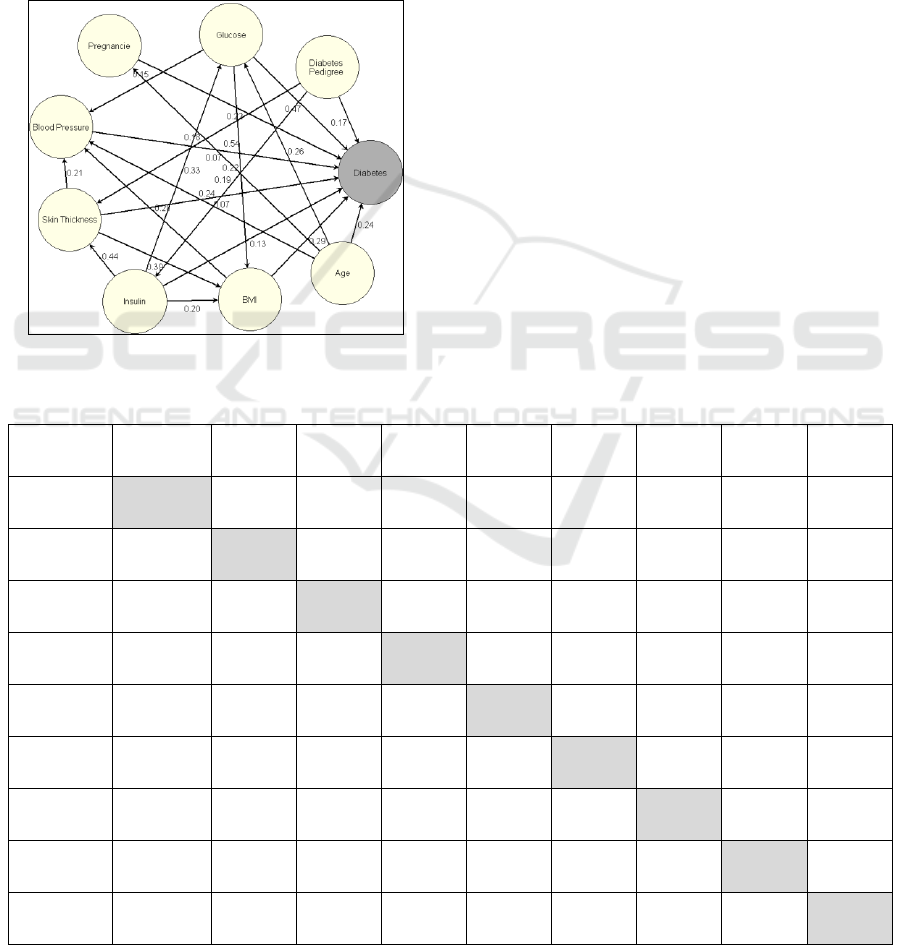
After identifying the significant values from the

correlation matrix, we employed two diabetologists

as domain experts in order to identify and confirm

causalities. The FCM model that emerged from this

process is shown in Figure 4 with the associated

edge-weight values.

Figure 4: Final FCM model for Diabetes dataset.

Similarly to the occupancy model, the constructed

FCM for the diabetes case is a full positive map

consisting exclusively of positive cycles. We

selected again the sigmoid function with λ=1, as the

threshold function and the update function given in

eq. (19).

A number of executions were performed on the

constructed model to assess its accuracy

performance. A number of 50 iterations were run for

each execution where the model managed to reach

equilibrium in all cases delivering a stable FCM

OUT

value. This value again was utilized by FCM-SVM

model and the execution results are presented and

discussed in Table 5.

4.5.2 Comparison

Table 5 presents the accuracy of the proposed

methodology compared to the baseline approaches.

As it can be seen, the best performing algorithms

from the baseline approaches are the Linear SVM

and the LDA that score 77.6%. The hybrid model

SVM-FCM scores again the higher accuracy with

78.65%, which, when compared against the k-NN,

LDA, Linear SVM and CT methods, yields an

average improvement of 2%.

Table 4: Correlation Matrix and p-values in parentheses for the diabetes dataset.

Pregnancy

Glucose

Blood

pressure

Skin

thickness

Insulin

BMI

Diabetes

Pedigree

Age

Pregnancy

0.00

0.129

(0.0003)

0.141

(8x10

-5

)

-0.081

(0.023)

-0.073

(0.041)

0.017

(0.624)

-0.033

(0.353)

0.544

(1x10

-60

)

0.221

(5x10

-10

)

Glucose

0.129

(0.0003)

0.00

0.152

(2x10

-5

)

0.057

(0.112)

0.331

(3x10

-21

)

0.221

(5x10

-10

)

0.137

(0.0001)

0.263

(1x10

-13

)

0.466

(8x10

-46

)

Blood

pressure

0.141

(8x10

-5

)

0.152

(2x10

-5

)

0.00

0.207

(6x10

-9

)

0.088

(0.013)

0.281

(1x10

-15

)

0.041

(0.253)

0.239

(1x10

-11

)

0.065

(0.071)

Skin

thickness

-0.081

(0.023)

0.057

(0.112)

0.207

(6x10

-9

)

0.00

0.436

(3x10

-37

)

0.392

(1x10

-29

)

0.183

(2x10

-7

)

-0.113

(0.001)

0.074

(0.038)

Insulin

-0.073

(0.041)

0.331

(3x10

-21

)

0.088

(0.013)

0.436

(4x10

-37

)

0.00

0.197

(3x10

-8

)

0.185

(2x10

-7

)

-0.042

(0.243)

0.130

(0.0002)

BMI

0.017

(0.624)

0.221

(5x10

-10

)

0.281

(1x10

-15

)

0.392

(1x10

-29

)

0.197

(3x10

-8

)

0.00

0.140

(9x10

-5

)

0.036

(0.315)

0.292

(1x10

-16

)

Diabetes

Pedigree

-0.033

(0.353)

0.137

(0.001

)

0.041

(0.253)

0.183

(2x10

-7

)

0.185

(2x10

-7

)

0.140

(9x10

-5

)

0.00

0.033

(0.352)

0.173

(1x10

-6

)

Age

0.544

(1x10

-60

)

0.263

(1x10

-13

)

0.239

(1x10

-11

)

-0.113

(0.0015)

-0.042

(0.243)

0.036

(0.315)

0.033

(0.352)

0.00

0.238

(2x10

-11

)

0.221

(5x10

-10

)

0.466

(8x10

-43

)

0.065

(0.071)

0.074

(0.038)

0.130

(0.0002)

0.292

(1x10

-16

)

0.173

(1x10

-6

)

0.238

(2x10

-11

)

0.00

ICEIS 2017 - 19th International Conference on Enterprise Information Systems

562

Table 5: Prediction Accuracy.

Approach

Test Dataset

Weighted k-NN

0.7344

LDA

0.7760

Linear SVM

0.7760

Classification

Tree

0.7448

SVM-FCM

0.7865

5 CONCLUSIONS

This paper proposed a new hybrid model that aims

to improve the accuracy of a real-time prediction

process by overcoming the difficulties faced in such

complex and multi-conflicting environments. The

proposed model couples Fuzzy Cognitive Maps

(FCM) and Support Vector Machines (SVM). The

former is constructed so that it can reveal

interrelationships between the inputs of a given

dataset and deliver a latent variable which is then

used by the SVM in conjunction with the rest of the

input factors to produce predictions.

Our experimentation with two different

problems, one for predicting room occupancy and

the other for proper classification of diabetes cases,

assisted to successfully answering the research

questions posed in the beginning of this study: RQ1

was adequately addressed by investigating and

demonstrating that FCMs are indeed able to model

multivariable environments with high levels of

complexity as the ones described in the two

application domains. RQ2 was also successfully

answered by showing that a FCM model is able to

transform the complicated relationships of a

multivariable environment into a single collective

output that, when used with the SVM model, it

increases the accuracy of the predictions produced.

The proposed methodology can be used in a wide

range of applications to improve the accuracy of a

system.

Although the experimental part cannot be

considered by any means thorough, the results

obtained may be considered as encouraging and

promising. Future work will concentrate on further

investigating and improving the hybrid model’s

performance. The application of the proposed

methodology on more real-world prediction

problems and datasets will provide useful feedback

for a better calibration of the hybrid model. Finally,

the transition from the semi-automatic to a fully-

automatic learning process will also be examined.

REFERENCES

Andreou, A.S., Mateou, N.H. & Zombanakis, G.A., 2005.

Soft computing for crisis management and political

decision making: the use of genetically evolved fuzzy

cognitive maps. Soft Computing, 9(3), pp.194–210.

Asuncion, A. & Newman, D., 2007. UCI machine learning

repository.

Bueno, S. & Salmeron, J.L., 2009. Benchmarking main

activation functions in fuzzy cognitive maps. Expert

Systems with Applications, 36(3 PART 1), pp.5221–

5229.

Candanedo, L.M. & Feldheim, V., 2016. Accurate

occupancy detection of an office room from light,

temperature, humidity and CO2 measurements using

statistical learning models. Energy and Buildings, 112,

pp.28–39.

Cortes, C. & Vapnik, V., 1995. Support-Vector Networks.

Machine Learning, 20(3), pp.273–297.

Gou, J. et al., 2012. A new distance-weighted k-nearest

neighbor classifier. J. Inf. Comput. Sci.

Iakovidis, D.K. & Papageorgiou, E., 2011. Intuitionistic

Fuzzy Cognitive Maps for Medical Decision Making.

IEEE Transactions on Information Technology in

Biomedicine, 15(1), pp.100–107.

Kandasamy, W.B.V. & Smarandache, F., 2003. Fuzzy

cognitive maps and neutrosophic cognitive maps,

Infinite Study.

Kosko, B., 1986. Fuzzy cognitive maps. International

Journal of Man-Machine Studies, 24(1), pp.65–75.

Kosko, B., 2010. Fuzzy Cognitive Maps: Advances in

Theory, Methodologies, Tools and Applications 1st ed.

M. Glykas, ed., Springer-Verlag Berlin Heidelberg.

Kosko, B., 1993. Fuzzy thinking: The new science of fuzzy

logic, Hyperion Books.

Kosko, B., 1992. Neural networks and fuzzy systems: a

dynamical approach to machine intelligence.

Englewood Cliffs. NJ: Prentice—Hall, 1(99), p.1.

Loh, W.-Y., 2011. Classification and regression trees.

Wiley Interdisciplinary Reviews: Data Mining and

Knowledge Discovery, 1(1), pp.14–23.

Mohandes, M.A. et al., 2004. Support vector machines for

wind speed prediction. Renewable Energy, 29(6),

pp.939–947.

Papageorgiou, E., 2013. Review study on Fuzzy Cognitive

Maps and their applications during the last decade.

Business Process Management, pp.828–835.

Papageorgiou, E.I. & Poczeta, K., 2015. Application of

fuzzy cognitive maps to electricity consumption

prediction. In 2015 Annual Conference of the North

American Fuzzy Information Processing Society

(NAFIPS) held jointly with 2015 5th World

Conference on Soft Computing (WConSC). IEEE, pp.

1–6.

A Hybrid Prediction Model Integrating Fuzzy Cognitive Maps with Support Vector Machines

563

Papageorgiou, E.I., Poczeta, K. & Laspidou, C., 2016.

Hybrid model for water demand prediction based on

fuzzy cognitive maps and artificial neural networks. In

2016 IEEE International Conference on Fuzzy

Systems (FUZZ-IEEE). IEEE, pp. 1523–1530.

Papageorgiou, E.I. & Salmeron, J.L., 2013. A review of

fuzzy cognitive maps research during the last decade.

IEEE Transactions on Fuzzy Systems, 21(1), pp.66–

79.

Shin, K.-S., Lee, T.S. & Kim, H., 2005. An application of

support vector machines in bankruptcy prediction

model. Expert Systems with Applications, 28(1),

pp.127–135.

Smith, J.W. et al., 1988. Using the ADAP Learning

Algorithm to Forecast the Onset of Diabetes Mellitus.

Proceedings of the Annual Symposium on Computer

Application in Medical Care, p.261.

McLachlan, G., 2004. Discriminant analysis and statistical

pattern recognition (Vol. 544). John Wiley & Sons.

Papageorgiou, E., Georgoulas, G., Stylios, C., Nikiforidis,

G. and Groumpos, P., 2006, October. Combining

fuzzy cognitive maps with support vector machines for

bladder tumor grading. In International Conference on

Knowledge-Based and Intelligent Information and

Engineering Systems (pp. 515-523). Springer Berlin

Heidelberg.

ICEIS 2017 - 19th International Conference on Enterprise Information Systems

564