Braking Strategy for an Autonomous Vehicle in a Mixed Traffic Scenario
Raj Haresh Patel, J
´
er
ˆ
ome H
¨
arri and Christian Bonnet
Communication Systems Department, EURECOM, 06904 Sophia-Antipolis, France
Keywords:
Collision Avoidance, Autonomous Vehicle, Manually Driven Vehicle, Vehicular Mobility, Braking Strategy,
IDM.
Abstract:
During the early deployment phase of autonomous vehicles, autonomous vehicles will share roads with con-
ventional manually driven vehicles. They will be required to adjust their driving dynamically taking into
account not only preceding but also following conventional manually driven vehicles. This paper addresses
the challenges of adaptive braking to avoid front-end and rear-end collisions, where an autonomous vehicle
is followed by a conventional manually driven vehicle. We illustrate via simulations the consequences of
independent braking in terms of collisions, on both autonomous and conventional vehicles, and propose an
adaptive braking strategy for autonomous vehicles to coordinate with conventional manually driven vehicles
to avoid front and rear-end collisions.
1 INTRODUCTION
Today autonomous vehicles are equipped with sen-
sing technologies involving cameras, radars, lidars,
etc. and/or communication technologies like Vehicle
to Vehicle (V2V) or Vehicle to Infrastructure (V2X).
Most of the work on autonomous vehicles is based on
coordinated control decision making for intersection
clearance, lane merging, etc. as found in a survey by
Torres (Rios-Torres and Malikopoulos, 2016) consi-
dering ideal circumstances. Now assume less than
ideal circumstances where an autonomous vehicle is
alerted to a potential collision with some delay and/or
coordination and negotiations with other vehicles fail
(leading to potential collisions). Such a scenario cre-
ates an emergency situation (Campos et al., 2014),
making it imperative to brake and to come to a halt
to avoid collisions. Thus, the objective changes from
coordinated control to safety critical braking.
Collision free braking becomes much more com-
plicated when a mix of autonomous and manually dri-
ven vehicles need to come to a halt. It is more li-
kely that an autonomous vehicle will have a manually
driven vehicle as its neighbour, either in front or be-
hind, because of the higher number of manually dri-
ven vehicles compared to autonomous vehicles. Thus
the above described scenario of collision free braking
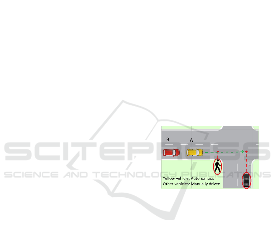
is an important concern today, as depicted in Figure 1
where vehicles A and B are autonomous and manually
driven respectively, and are trying to avoid collision
with a potential obstacle L in front by braking.
Figure 1: Mixed vehicular traffic scenario involving auto-
nomous and manually driven vehicles.
More than one-fifth of accidents happen with a
vehicle immediately behind or ahead in longitudinal
direction (Kaempchen et al., 2009), primarily be-
cause human drivers tend to react based on the vehi-
cle in front and prevent accidents with the vehicle in
front (front-end accident avoidance). Generally spea-
king, the effect of the braking of a vehicle onto the
following vehicle is not considered by humans lea-
ding to rear-end collisions. On the other hand, an au-
tonomous vehicle can consider potential collisions at
both ends. If the following vehicle and ego vehicle are
both autonomous, a coordinated braking strategy can
be devised. Consider the scenario where a conven-
tional manually driven vehicle without any form of
automation is following an autonomous vehicle (ego
vehicle). The objective of this paper is to answer the
following question: How can an autonomous vehi-
cle anticipate the braking of a following conventional
vehicle, modify its controls considering the (anticipa-
268
Patel, R., Härri, J. and Bonnet, C.
Braking Strategy for an Autonomous Vehicle in a Mixed Traffic Scenario.
DOI: 10.5220/0006307702680275
In Proceedings of the 3rd International Conference on Vehicle Technology and Intelligent Transport Systems (VEHITS 2017), pages 268-275
ISBN: 978-989-758-242-4
Copyright © 2017 by SCITEPRESS – Science and Technology Publications, Lda. All rights reserved

ted) braking of the following vehicle and guarantee
both rear-end and front-end collision avoidance (with
the following vehicle and with the obstacle in front
respectively) in the above described scenario.
Our contributions are threefold: first we formulate
a collision free adaptive (cooperative) braking stra-
tegy as a multi-parameter objective based on braking
distances and dynamics of following conventional
vehicles; second, we propose an adaptive ‘smooth’
braking strategy for autonomous vehicles and demon-
strate its capability to avoid rear and front-end colli-
sions. Finally, we vary the input parameters to illus-
trate their impact on our proposed coordinated bra-
king strategy.
The rest of this paper is organized as follows: in
Section 2, we formulate the coordinated braking pro-
blematic with more details and provide related work.
In Section 3 we provide a detailed modelling of it,
whereas in Section 4 we evaluate our proposed stra-
tegy. Finally, Section 5 concludes our work and sheds
light on future work.
2 RELATED WORK
In this paper we use various braking strategies and
vehicular mobility models to simulate different sce-
narios for front-end and rear-end collision avoidance
in longitudinal motion. First subsection looks at the
work related to vehicular mobility models and bra-
king strategies whereas the latter part of this section
looks at work related to collision avoidance.
2.1 Vehicular Mobility Models
In literature, there are lots of vehicular mobility mo-
dels. Psycho-physical model by Wiedemann (Wie-
demann, 1974), is one such mobility model imple-
mented in VISSIM simulator (Fellendorf and Vor-
tisch, 2010). It states that a manually driven vehicle
is in one of the following driving modes: free driving,
approaching, following or braking. An approaching
vehicle would continue at the same velocity until it
enters a deceleration perceptual threshold which sti-
mulates the driver to brake. Whereas Trebier proposes
Intelligent Driver Model (IDM) (Treiber et al., 2000)
in which he suggests that the ego vehicle adjusts its
driving dynamics according to that of the vehicle im-
mediately in front to avoid front-end collisions. Sub-
sequent extensions of IDM like Enhanced IDM (Kes-
ting et al., 2010a) and IDM+ (Schakel et al., 2010)
optimizes traffic capacity and flow. In such Follow-
the-Leader models the presence of following vehicles
is not considered leaving a big risk of rear-end colli-
sions.
1
Kesting assumes IDM or a modified version of
IDM to be a good basis for implementation of
Adaptive Cruise Control (ACC)/ Cooperative ACC
(CACC) (Kesting et al., 2010b), thus we assume
in this paper, autonomous vehicles implement IDM.
IDM can be modelled as in equation 1.
a
α
= a
max
(1 −(
v
α
v
0
)
δ
−(
s
∗
(v
α
,∆v
α
)
s
α
)
2
)
s
∗
(v
α
,∆v
α
) = s
0
+ v
α
τ +
v
α
∆v
α
2
√
a
max
b
max
s
α
= x
α−1
−x
α
−l
α−1
∆v
α
= v
α
−v
α−1
(1)
Where α is the vehicle being considered, α −1 is the
vehicle in front and so on. a
α
,v
α
,x
α
represents acce-
leration, velocity and the location of vehicle α. a
max
,
b
max
are maximum acceleration and braking values of
the vehicle. s
α
, ∆v
α
, τ represent distance, velocity dif-
ference and desired time gap with the vehicle in front.
δ is the free acceleration exponent. s
0
is the desired
safety distance between two vehicles and v
0
is the de-
sired velocity of vehicle in free traffic. l
α−1
is the
length of the vehicle α −1.
On the other hand, human drivers in manually dri-
ven vehicles are assumed to show realistic characte-
ristics like having a reaction to a situation after some
perception response time t
prt
. In other words, t
prt
is
the measure of attentiveness and responsiveness of a
driver. When travelling at high speeds, and noticing
the vehicle in front close and braking, humans would
tend to immediately hit the brakes. We assume, as this
situation is a sudden surprise, the magnitude of app-
lied brakes is maximum. In this paper, we set the va-
lue of t
prt
to 1.3 s, which is the mean value of human
perception response time (National Highway Traffic
Safety Administration, 2009). To summarize, manu-
ally driven vehicles are assumed to brake at maximum
braking strength, 1.3 s after the vehicle in front starts
braking until they come to a halt. In future, autono-
mous vehicles with sensors could learn about the t
prt
of the driver in vehicle behind based on the observed
driving behaviour.
2.2 Collision Avoidance Strategies
Most of the work till date has been on collision avoi-
dance between ego vehicle and vehicle in front and
1
Through simulations we show a rear-end collision of
an autonomous vehicle with a manually following vehicle.
Refer to Figure 11, explained in Subsection 4.2.
Braking Strategy for an Autonomous Vehicle in a Mixed Traffic Scenario
269

Figure 2: Simplified 1D scenario where autonomous vehi-
cle A detects an obstacle L via V2X communication.
comparatively little on the influence of actions of ego
vehicle onto following vehicle.
To avoid front-end collisions, for manually driven
vehicles, traditionally proposed solution is to have
larger inter vehicular distances, (Ashley, 2013) sta-
tes the recommended headway in Germany is 1.8
s. For vehicles with V2V communication capacities,
(Liu and Ozguner, 2003) suggests increasing com-
munication range to warn about a potential collision
over a larger range. Where as for autonomous vehi-
cles, (Llorca et al., 2011; Durali et al., 2006) pro-
pose front-end collision avoidance based on steering
rather than braking. Brandt proposes an innovative
elastic band theory based approach involving non li-
near algebraic equations for collision avoidance sy-
stems (Brandt et al., 2005). Intent prediction based
front-end collision avoidance is proposed by Hamlet
in (Hamlet et al., 2015). An approach for collision
avoidance during automated lane changing is presen-
ted by (Jula et al., 2000). Lu proposes a centralized
coordinated braking strategy for ACC vehicles using
Model Predictive Control (Lu et al., 2014).
On the other end, to avoid rear-end collisions,
either the following vehicle should be informed as to
when by latest it should start braking as suggested by
Zhang (Zhang et al., 2006) or leading vehicle should
be informed the latest moment by when it must acce-
lerate as suggested by Cabrera (Cabrera et al., 2012).
All the cited work assumes homogeneous traffic
with vehicles having the same level of automation.
Little attention has been given to rear-end collision
avoidance as evident from above. Most of the ac-
complished work, requires V2V communication to in-
form neighbouring vehicles about control strategies.
What happens when the following vehicle doesn’t
have neither any V2V communication nor sensing
technology? Are collisions inevitable?
3 MODELLING ADAPTIVE
BRAKING STRATEGY
Without loss of generality, we simplify the scenario
described in Figure 1, consisting of a potential ob-
stacle L, an autonomous vehicle A and a manually
Figure 3: Relation between ∆t and T
range
.
driven vehicle B following A, to a 1D representation
in Figure 2. d
e
, d
la
represents the distance cove-
red during an emergency brake at maximum braking
strength by vehicle A and the distance at which vehi-
cle A becomes aware of the potential danger by object
L over V2X communication respectively. We assume
d
la
is strictly bigger than the sensing range of vehi-
cle A’s sensors. WiFi-based ITS-G5/DSRC techno-
logy communicating over a 5.9GHz frequency band
(V2X/V2V), usually has a communication range(d
la
)
of a few hundred meters, but harsh communication
conditions (i.e. Non-Line-of-Sight, channel conges-
tion. . . ) restricts this range d
la
. We consider in this
paper d
la
to be strictly bigger than d
e
(d
la
> d
e
), so
that vehicle A may use the distance d
s
= d
la
−d
e
to
adjust its braking strategy. d
ab
is distance between A
and B.
To ensure collision avoidance at both ends, we pro-
pose a braking strategy for leading vehicle A (ego
vehicle) consisting of two phases: weak and hard. We
illustrate this concept with Figure 3. T is the time
any vehicle takes to come to a full halt once it starts
braking (T
a
is the time vehicle A takes to come to a
full halt), and covers a distance shorter than d
la
. The
weak braking time interval is represented as T
weak
,
which lasts for ∆t s, during which the vehicle will gra-
dually increase its braking magnitude from zero and
eventually reach maximum braking strength. Beyond
T
weak
, for a duration of T −T
weak
s, the vehicle main-
tains maximum braking strength until it comes to a
halt. This time duration is the hard braking phase.
The challenge is to determine the braking duration ∆t
which signals the shift from weak to hard braking ma-
noeuvre. ∆t is not unique and can take multiple values
within a time interval T
range
[t
low
,t
up
] as shown in Fi-
gure 3. t
up
corresponds to an upper bound to avoid
collision with obstacle L and t
low
corresponds to a lo-
wer bound to avoid collision with vehicle B. The same
is derived next.
To determine the values of t
up
and t
low
, we ana-
lyse the deceleration behaviour of vehicles A and B
in Figure 4. This image can be understood by de-
composing the braking manoeuvres of both vehicles
into four phases (or intervals): Phase A, corresponds
to vehicle B’s reaction time during which it doesn’t
brake where as vehicle A is in weak braking phase.
Phase B, is the time after t
prt
, when vehicle A is still
VEHITS 2017 - 3rd International Conference on Vehicle Technology and Intelligent Transport Systems
270
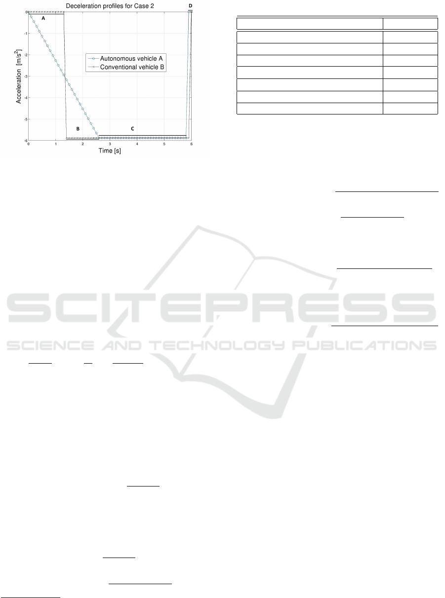
Figure 4: Deceleration profile of vehicles.
in weak braking phase and vehicle B has started to
brake at maximum strength. Phase C corresponds to
both vehicles braking hard, while phase D is when
both vehicles come to a halt (collision or not).
2
Now,
to ensure collision-free ride, the following conditions
need to be ensured:
#1 – d
la
> 0 to avoid front-end collision: corresponds
to upper bound of T
range
(t
up
)
#2 – d
ab
> 0 to avoid rear-end collision: corresponds
to lower bound of T
range
(t
low
)
Ensuring #1: Total distance covered by vehicle A
before halting must be smaller than initial distance
d
la(t=0)
. (L is stationary in longitudinal direction).
Simplifying kinematic equations for #1 we get:
∆t
2
(
b
max,a
24
) + ∆t (
v
a
2
) + (
v
2
a
2 b
max,a
−d
la(t=0)
) < 0
(2)
where v
a
is the initial velocity and b
max,a
is the maxi-
mum braking strength of vehicle A.
Ensuring #2: As vehicles A and B behave differently
in different time phases, but within a phase their bra-
king behaviour remains constant, we split our analysis
for #2 into four intervals previously described:
• Interval A: t ∈ [0,t
prt
)
d
ab
(t) = d
ab(t=0)
+
b
max,a
t
3
6 ∆t
> 0 (3)
where d
ab(t=0)
is the initial distance between vehi-
cles A and B.
• Interval B: t ∈ [t
prt
,∆t)
d
ab
(t) = d
ab(t=0)
+
b
max,a
t
3
6 ∆t
−
b
max,b
(t −t
prt
)
2
2
> 0 (4)
2
Not always would both vehicles come to a halt at the
same time
Table 1: IDM constants and their values.
Parameter description value
Desired speed (v
0
) 96 km/h
Free acceleration exponent (δ) 4
Desired time gap (τ) 0.1 s
Maximum acceleration (a
max
) 1.4 m/s
2
Maximum braking strength (b
max
) -0.6g m/s
2
Length of vehicle (l
a
) 4 m
Desired minimum distance (s
0
) 5 m
where b
max,b
is the maximum braking strength of
vehicle B.
• Interval C: t ∈[∆t,T = min(T
a
,T
b
) or T = T
a
= T
b
]
d
ab
(t) = d
ab(t=0)
+
b
max,a
(∆t
2
−3 t ∆t −3 t
2
)
6
−
b
max,b
(t −t
prt
)
2
2
> 0 (5)
• Interval D: t ∈ [T
a
,T
b
] ... for T
b
> T
a
:
d
ab
(t) = d
ab(t=T )
+ (
(v
b
+ b
max,b
(T
a
−t
prt
))
2
2 b
max,b
)
(6)
or interval t ∈[T
b
,T
a
]... for T
b
< T
a
:
d
ab
(t) = d
ab(t=T )
−(
(v
a
+ b
max,a
(T
b
−0.5 ∆t))
2
2 b
max,a
)
(7)
where d
ab(t=T )
is the distance between vehicles A and
B at time T .
Solving equations mentioned under #1 and #2 re-
turn a set of possible values which define the time
interval T
range
. The value ∆t (between t
low
and t
up
)
that vehicle A takes depends on its driving strategy
but this is out of scope of this paper. The mean
value is being taken by default in our calculations:
∆t = (t
up
−t
low
)/2.
4 PERFORMANCE EVALUATION
We split our experiment into two cases implementing
three braking strategies:
Case 1. Vehicle A implements IDM whereas vehicle
B implements human behaviour (manual braking)
Case 2. Vehicle A implements the proposed braking
strategy whereas vehicle B implements human beha-
viour (manual braking)
IDM and manual braking were introduced in
Section 2 and the new proposed strategy was intro-
duced in Section 3. Values of different parameters
Braking Strategy for an Autonomous Vehicle in a Mixed Traffic Scenario
271
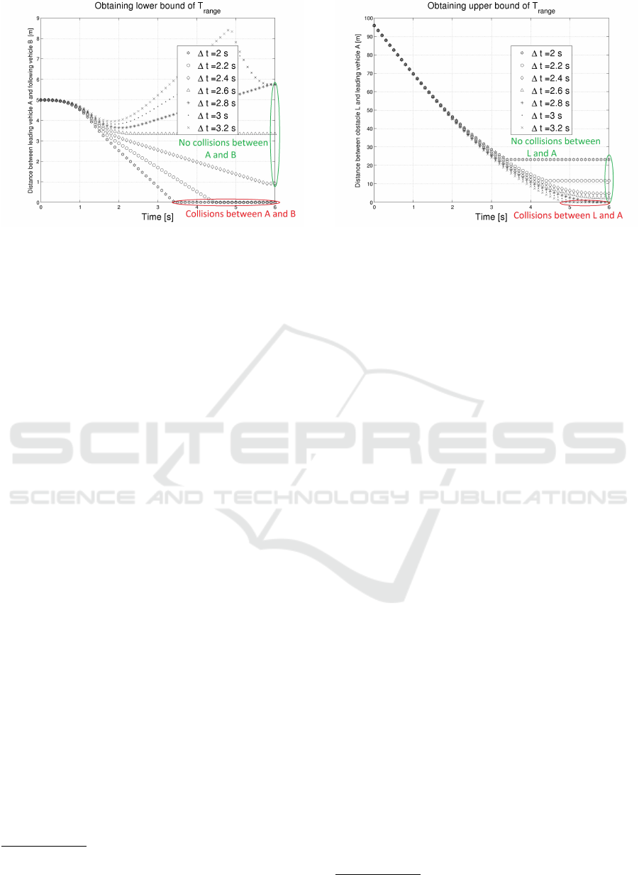
Figure 5: Calculating lower bound for T
range
.
used in IDM are summarized in Table 1.
3
We eva-
luate using Matlab proposed braking strategy against
IDM by analysing these two cases.
4.1 Adaptive Braking Strategy
In order to illustrate the role of different parameters
influencing T
range
in the proposed approach, we consi-
der three sets of evaluations: (I) we fix all parameters
and focus on choosing the right value of ∆t; (II) we
change initial speed of the vehicles and keep rest of
the parameters as before; (III) we consider the influ-
ence of environmental and road conditions (ice, rain,
etc..).
Using An’s work (An et al., 2011) we calculate
that by the time distance reduces to 95.9 m from trans-
mitter of the emergency notification message, recei-
ver can be assumed to have received at least one
emergency message with 99.5% probability. We thus
set d
la
= 95.9 m. For (I) set of evaluation, we fix:
d
ab
= 5m, length of vehicle A (l
a
) is 4 m, Initial velo-
cities of both vehicles A (v
a
) and B (v
b
) are assumed
to be equal v
0
= v
a
= v
b
. For a highway scenario we
assume v
0
= 96 km/h. Moreover we assume that both
vehicles A and B can reach a maximum braking capa-
city (b
max
) of −0.6g, which is the mean of maximum
deceleration strengths of vehicles (National Highway
Traffic Safety Administration, 2002), g is gravitatio-
nal constant 9.88m/s
2
.
Set of equations 2- 7 can be used to derive the va-
lue T
range
= [2.4,2.8] s, refer Table 2. The same range
can also be obtained graphically. For different ∆t va-
lues, Figure 5 illustrates the variation of d
ab
vs time
where as Figure 6 illustrates the variation of d
la
vs
time. Intersection of a plot with x-axis indicates zero
3
For emergency braking situations like the one conside-
red here, limitations on jerks or comfort are not considered
for analytical calculations
Figure 6: Calculating upper bound for T
range
.
distance between vehicles. Thus ∆t should be cho-
sen such that the plot doesn’t intersect x-axis in Fi-
gure 5, 6. The Upper bound t
up
can be determined
visually from Figure 6 (thus #1 resolved), while the
Lower bound t
low
can be determined visually from Fi-
gure 5 (thus #2 is resolved). Now, a value ∆t can be
chosen: ∆t ∈ T
range
; T
range
= [t
up
,t
down
].
Note: in Figure 5, plots for ∆t > 2.8 s converge to
the same point as seen, because A has collided with L
and B comes to halt at the same position; thus d
ab
at
the end of simulations for ∆t > 2.8 s is the same.
To further illustrate the consequences of an in-
accurate ∆t, we consider three different possibilities
in Figure 7. The first possibility corresponds to con-
ditions on ∆t are not respected, and ∆t is chosen smal-
ler than the acceptable T
range
. In this case, it can be
seen that A collides with B (i.e. rear-end collision for
(∆t < t
low
)).The second possibility corresponds to the
desired scenario where ∆t is chosen from the calcula-
ted T
range
, and collisions are avoided (i.e. ∆t ∈T
range
).
The third possibility corresponds to the case, where ∆t
is too big and A fails to brake and collides into L (i.e.
front-end collision for ∆t > t
up
).
For (II) set of evaluation, we change the initial
velocities of vehicle v
0
(v
a
= v
b
), keeping the same
d
ab
= 5 m. The objective is to find the minimum d
la
and the corresponding T
range
for ∆t to be used by vehi-
cle A to avoid any collisions. Results are summarized
in Table 3.
4
Approaches used in evaluations (I) and (II) as-
sume decent road conditions. If a road surface with
some oil or sand spill (dirty) is considered, maximum
deceleration is physically restricted to −4 m/s
2
(Bar-
bier, 2013). In (III) set of evaluation, we limit bra-
king capacity to −4 m/s
2
. Simulations show if the
vehicles are travelling at 96 km/h with d
ab
= 5 m, and
d
la
= 95.9 m collisions can not be averted (i.e. A will
4
x denotes either a rear-end or a front-end collision
VEHITS 2017 - 3rd International Conference on Vehicle Technology and Intelligent Transport Systems
272
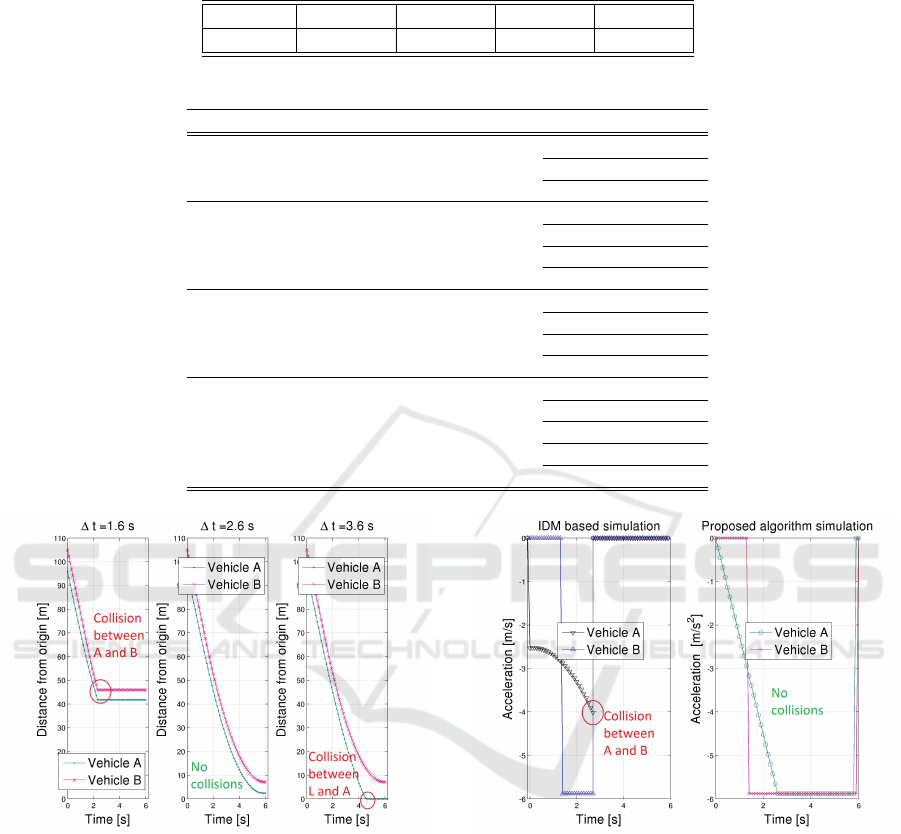
Table 2: Distance between autonomous and conventional vehicle and corresponding time to reach maximum deceleration for
v = 96km/h; d
la
(t = 0) = 95.9m; highway scenario.
d
ab
[m] 5 8 10 15
T
range
[s] 2.4 to 2.8 2.1 to 2.8 2.0 to 2.8 1.6 to 2.8
Table 3: T
range
corresponding to braking strategies for different vehicular speed.
Velocity [km/h] d
la
[m] T
range
[s]
v
0
= 30; low speed limit scenario
10 x
15 1.6 to 2.5
20 1.6 to 4.6
v
0
= 50; urban city with stricter speed limits
20 x
30 2.1 only
35 2.1 to 2.9
40 2.1 to 3.9
v
0
= 70; urban city scenario
50 x
55 2.3 to 2.5
60 2.3 to 3.1
70 2.3 to 4.3
v
0
= 96; highway scenario
90 x
95.9 2.4 to 2.8
100 2.4 to 3.1
110 2.4 to 4
120 2.4 to 4.9
Figure 7: Three cases - rear-end collision, no collision,
front-end collision.
collide with either B or L). For these reasons, the max-
imum speed limit should be capped, say to 80 km/h
(50 mph) which in turn returns T
range
of [2.3,3.2]
s. Alternately, under optimal road conditions which
could support braking up to −8 m/s
2
, maximum velo-
city permitted can be increased up to 110 km/h (68
mph) such that with ∆t values of [2.3,2.4] s, collisi-
ons could be avoided.
Figure 8: Acceleration profile of vehicles; vehicle A follo-
wing: IDM (left) proposed algorithm (right).
4.2 Adaptive vs. IDM-ACC Braking
We complete our evaluation with a comparison of
adaptive braking strategy (proposed algorithm, imple-
mented in Case 2) against the IDM-ACC mechanism
(implemented in Case 1) for the same set of parame-
ters. Sub-plots on the right of Figures [8, 9, 10] de-
monstrates the performance of our algorithm compa-
red to IDM’s on the left; these plots highlight accele-
ration, velocity and location comparison between the
two. IDM would demand an instantaneous increase
Braking Strategy for an Autonomous Vehicle in a Mixed Traffic Scenario
273
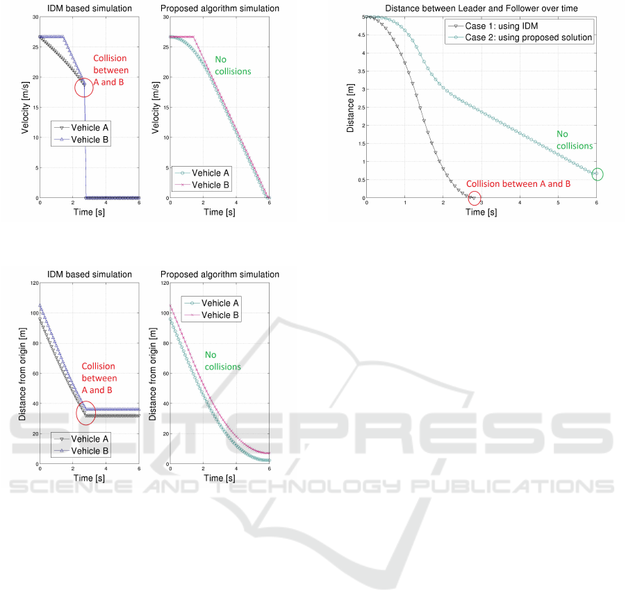
Figure 9: Velocity profile of vehicles; leading vehicle follo-
wing: IDM (left) proposed algorithm (right).
Figure 10: Locations of vehicles; leading vehicle following:
IDM (left) proposed algorithm (right).
in braking strength from zero (to -2.5 m/s
2
approxi-
mately in this case) as shown in Figure 8 where as
the proposed approach is more comfortable as bra-
king strength is increased gradually. At 2.8 seconds,
the acceleration jumps from around -4 to 0 m/s
2
in the
plot on the left in Figure 8, which is due to rear-end
collision of vehicle A with B. Same is the interpreta-
tion of Figure 9 which shows sudden fall of velocity
to zero after the accident between A and B. Figure
10 shows the vehicles maintaining their position af-
ter collision at 2.8 s. Whereas the plot on the right of
Figures [8, 9, 10] show smooth collision free braking.
Finally, from Figure 11 it is clear that front-
end collisions could be avoided but rear-end accident
could not be avoided as d
ab
reaches zero for Case 1,
where as the proposed braking strategy implemented
in Case 2 avoids accidents at both ends. These figures
clearly supports our claim that IDM indeed couldn’t
assure collision avoidance of the following vehicle
onto itself where as our proposed algorithm does.
Figure 11: Inter-distance between vehicle A and B.
5 CONCLUSIONS
When an autonomous vehicle needs to suddenly
brake, it should consider not only the possible front-
end collision, but also rear-end collision with the fol-
lowing vehicle. In this paper, we address this aspect
and propose a braking strategy for a scenario invol-
ving a manually driven vehicle following an autono-
mous vehicle. First phase of the braking avoids hard
brake where as a second phase performs a conventio-
nal hard brake.
The proposed approach also suggests that even at
high velocities (96km/h) and low inter vehicular dis-
tance (5m), safety is not compromised provided the
autonomous vehicle gradually increases its braking
strength to maximum. Most importantly, via simu-
lation, we show the superiority of the proposed algo-
rithm over ACC/CACC algorithms like IDM in bra-
king circumstances, which usually only manages to
avoid front-end collision at the cost of a rear-end col-
lision.
Future work will focus on developing a control
theory based approach which would provide control
inputs for coordinated braking of multiple vehicles
with different levels of automation in a heterogeneous
traffic scenario, whilst optimizing a particular cost
function.
ACKNOWLEDGEMENTS
Raj Haresh Patel is a recipient of a PhD Grant from
the Graduate School of the University Pierre Ma-
rie Curie (UPMC), Paris. EURECOM acknowledges
the support of its industrial members, namely, BMW
Group, IABG, Monaco Telecom, Orange, SAP, ST
Microelectronics, and Symantec.
VEHITS 2017 - 3rd International Conference on Vehicle Technology and Intelligent Transport Systems
274

REFERENCES
An, N., Gaugel, T., and Hartenstein, H. (2011). Vanet: Is
95% probability of packet reception safe? In ITS Tele-
communications (ITST), 2011 11th International Con-
ference on, pages 113–119.
Ashley, S. (2013). Truck platoon demo reveals 15% bump
in fuel economy. accessed 02-March-2016.
Barbier, M. (2013). Experienced network access selection
with regards to safety applications. Master’s Thesis,
EURECOM.
Brandt, T., Sattel, T., and Wallaschek, J. (2005). On auto-
matic collision avoidance systems. pages 316–326.
Cabrera, A., Gowal, S., and Martinoli, A. (2012). A new
collision warning system for lead vehicles in rear-end
collisions. In 2012 IEEE Intelligent Vehicles Sympo-
sium, pages 674–679.
Campos, G. R., Falcone, P., Wymeersch, H., Hult, R., and
Sj
¨
oberg, J. (2014). Cooperative receding horizon con-
flict resolution at traffic intersections. In 53rd IEEE
Conference on Decision and Control, pages 2932–
2937. IEEE.
Durali, M., Javid, G. A., and Kasaiezadeh, A. (2006). Colli-
sion avoidance maneuver for an autonomous vehicle.
In 9th IEEE International Workshop on Advanced Mo-
tion Control, 2006., pages 249–254.
Fellendorf, M. and Vortisch, P. (2010). Microscopic traf-
fic flow simulator vissim. In Fundamentals of traffic
simulation, pages 63–93. Springer.
Hamlet, A. J., Emami, P., and Crane, C. D. (2015). The cog-
nitive driving framework: Joint inference for collision
prediction and avoidance in autonomous vehicles. In
Control, Automation and Systems (ICCAS), 2015 15th
International Conference on, pages 1714–1719.
Jula, H., Kosmatopoulos, E. B., and Ioannou, P. A. (2000).
Collision avoidance analysis for lane changing and
merging. IEEE Transactions on Vehicular Techno-
logy, 49(6):2295–2308.
Kaempchen, N., Schiele, B., and Dietmayer, K. (2009).
Situation assessment of an autonomous emergency
brake for arbitrary vehicle-to-vehicle collision scena-
rios. IEEE Transactions on Intelligent Transportation
Systems, 10(4):678–687.
Kesting, A., Treiber, M., and Helbing, D. (2010a). En-
hanced intelligent driver model to access the impact
of driving strategies on traffic capacity. Philosophi-
cal Transactions of the Royal Society of London A:
Mathematical, Physical and Engineering Sciences,
368(1928):4585–4605.
Kesting, A., Treiber, M., and Helbing, D. (2010b). En-
hanced intelligent driver model to access the impact
of driving strategies on traffic capacity. Philosophi-
cal Transactions of the Royal Society of London A:
Mathematical, Physical and Engineering Sciences,
368(1928):4585–4605.
Liu, Y. and Ozguner, U. (2003). Effect of inter-vehicle com-
munication on rear-end collision avoidance. In Intel-
ligent Vehicles Symposium, 2003. Proceedings. IEEE,
pages 168–173.
Llorca, D. F., Milanes, V., Alonso, I. P., Gavilan, M., Daza,
I. G., Perez, J., and Sotelo, M. . (2011). Autonomous
pedestrian collision avoidance using a fuzzy steering
controller. IEEE Transactions on Intelligent Transpor-
tation Systems, 12(2):390–401.
Lu, X.-Y., Wang, J., Li, S. E., and Zheng, Y. (2014).
Multiple-vehicle longitudinal collision mitigation by
coordinated brake control. Mathematical Problems in
Engineering, 2014.
National Highway Traffic Safety Administration (2002).
Alert Algorithm Development Program: NHTSA
Rear-End Collision Alert Algorithm. Contract No:
DTFH61-99-C-00051, DOT HS 809 526.
National Highway Traffic Safety Administration (2009).
Development of an FCW Algorithm Evaluation Met-
hodology with Evaluation of Three Alert Algorithms.
Contract No: DTFH61-99-C-00051, DOT HS 811
145.
Rios-Torres, J. and Malikopoulos, A. A. (2016). A sur-
vey on the coordination of connected and automated
vehicles at intersections and merging at highway on-
ramps. IEEE Transactions on Intelligent Transporta-
tion Systems.
Schakel, W. J., van Arem, B., and Netten, B. D. (2010). Ef-
fects of cooperative adaptive cruise control on traffic
flow stability. In Intelligent Transportation Systems
(ITSC), 2010 13th International IEEE Conference on,
pages 759–764. IEEE.
Treiber, M., Hennecke, A., and Helbing, D. (2000). Con-
gested traffic states in empirical observations and mi-
croscopic simulations. Physical review E, 62(2):1805.
Wiedemann, R. (1974). Simulation des strassenverkehrs-
flusses.
Zhang, Y., Antonsson, E. K., and Grote, K. (2006). A new
threat assessment measure for collision avoidance sy-
stems. In 2006 IEEE Intelligent Transportation Sys-
tems Conference, pages 968–975.
Braking Strategy for an Autonomous Vehicle in a Mixed Traffic Scenario
275
