Pedestrian Tracking using a Generalized Potential Field Approach
Florian Particke
1
, Lucila Pati
˜
no-Studencki
1
, J
¨
orn Thielecke
1
and Christian Feist
2
1
Information Technologies, Friedrich-Alexander-Universit
¨
at Erlangen-N
¨
urnberg (FAU),
Am Wolfsmantel 33, 91058 Erlangen, Germany
2
Audi Electronics Venture GmbH, 85080 Gaimersheim, Germany
Keywords:
Object Tracking, Pedestrians, Surveillance, Pedestrian Trajectory Pattern, Parametric Model.
Abstract:
Mobile robots and autonomous driving cars operate in a shared environment with pedestrians. In order to
avoid accidents, it is important to track and predict human trajectories in an optimal way. In this paper, a
generalized potential field approach for characterizing pedestrian movements is proposed which goes beyond
the well-known social force model. Its goal is to give a generalized architecture for improving the tracking
accuracy of pedestrians in surveillance situations. In comparison to other fusion approaches, the number of
proposed parameters is reduced and the parameters can be intuitively understood. For a simple scenario, in
a forum the trajectories of pedestrians are predicted for a configured parameter set. For this purpose, the
proposed model is used. The predicted trajectories are compared to the real trajectories of the pedestrians.
First results regarding the accuracy of the approach are presented.
1 INTRODUCTION
In the field of robotics and autonomous driving cars
vehicles or robots often have to interact with pedestri-
ans. To assure that the risk for pedestrian is minimal,
it is very important to track pedestrians in a precise
way. Camera based sensors are mostly used in closed
rooms, especially in surveillance areas. Tracking of
dynamic objects by cameras is a recent research topic
(Ibisch et al., 2015).
To improve tracking accuracy, many different
models for pedestrians have been proposed over the
last decades. Fluid-dynamic models were used to de-
scribe the macroscopic behavior of pedestrians. In
(Helbing, 1998) a Boltzmann-like gas-kinetic model
was introduced, which was motivated by good results
in traffic flow simulation (Alberti and Belli, 1978;
Prigogine, 1900), but the model neglects the individ-
ual behavior of pedestrians. In the microscopic field,
Markovian models were developed to differentiate be-
tween different pedestrians states like standing, walk-
ing and running (Wakim et al., 2004). For compu-
tational issues, grid cell based approaches were in-
troduced (Dijkstra et al., 2001), which are based on
the class of cell automata models. A specialization
of this class is the floor field approach (Ali and Shah,
2008), which combines the interaction of pedestrians
in crowded scenes with the environment. For the floor
field approach, frameworks of pedestrian crowd sim-
ulation were developed (Kretz and Schreckenberg,
2006). Another microscopic and physical approach is
the social force model (Dirk Helbing and Peter Mol-
nar, 1995), which describes every human interacting
in a field of social forces. These social forces are de-
fined by other pedestrians and the environment. The
social force model proposes every pedestrian aims to
have an individual velocity in a certain direction.
Beside the proposed models, an extensive research
in using the different information sources for predict-
ing trajectories or improving the tracking of pedestri-
ans is performed. Recent research often focuses on
intention prediction (Bandyopadhyay et al., 2013b;
Bandyopadhyay et al., 2013a) for optimal motion
planning or the decision process of crossing the street
(Keller and Gavrila, 2014). Other research is based
on dynamic object interactions and planning (Heine-
mann et al., 2006). But often only one or two informa-
tion sources (e.g. intention or environment) are con-
sidered and the approaches can not easily be general-
ized.
Frameworks, which give a generalized architec-
ture for the fusion of many information sources typi-
cally consist of settings with many parameters. These
parameters often can not be intuitively understood
and have to be trained by machine learning algo-
rithms. Typical examples of approaches with at least
ten parameters are (Heinemann et al., 2006; Robin
et al., 2009; Yi et al., 2015). In this paper, a phys-
Particke F., PatiÃ
´
so-Studencki L., Thielecke J. and Feist C.
Pedestrian Tracking using a Generalized Potential Field Approach.
DOI: 10.5220/0006215705090514
In Proceedings of the 12th International Joint Conference on Computer Vision, Imaging and Computer Graphics Theory and Applications (VISIGRAPP 2017), pages 509-514
ISBN: 978-989-758-227-1
Copyright
c
 2017 by SCITEPRESS – Science and Technology Publications, Lda. All rights reserved
509

ical model based on the social force model is moti-
vated, which tries to minimize the number of parame-
ters. Furthermore, the value of the parameters doesn’t
have to be learned by trajectories of real scenarios, but
can be intuitively understood and configured.
This paper is organized as follows. In section 2 the
model is proposed, in section 3 a pedestrian prediction
model is derived, which includes the proposed dy-
namical model. With this pedestrian prediction model
trajectories are generated, which are compared with
real observed trajectories. The evaluation is discussed
in section 4, in section 5 further steps of future re-
search are presented.
2 PROPOSED MODEL
The model is driven by the idea to improve clas-
sic tracking algorithms like Kalman Filter or Monte
Carlo Methods through the fusion of available infor-
mation sources. These information sources could be
the environment, dynamic object interactions, inten-
tion, that are the goals of the pedestrians (Tamura
et al., 2012) or crowd effects (Yi et al., 2015). The
model is based on the assumption that pedestrians act
like test particles in a potential field. The goal of the
model is the calculation of the person’s acceleration
resulting from the corresponding potential field.
2.1 Calculation of Potential Field
As mentioned before, every pedestrian acts like a test
particle in each potential field. Each potential field φ
k
represents an information source (e.g. enviroment is
represented as a map) and is the combination of n
k
potential sources φ
k
i
(e.g. wall in the map). The po-
tential at the position of the pedestrian is calculated
by the weighted sum of φ
k
i
potentials, which can be
interpreted as contour lines, at the position P
k
(x
i
,y
i
)
in the distance d
k
iN
between the pedestrian and the po-
tential source φ
k
i
. The potential φ
k
N
at the position of
the pedestrian P
N
(x
N
,y
N
) with the weight p
k
can be
interpolated according to (Niemeier, 2008, S. 411).
The weight p
k
is assumed to be dependent on the dis-
tance to the pedestrian d
k
iN
, but independent of time.
φ
k
N
=
n
k
∑
i=1
p
k
(d
k
iN
)φ
k
i
(1)
The distance d
k
iN
to the pedestrian in two dimen-
sional space is calculated by the euclidean distance:
d
k
iN
=
q
(x
k
i
− x
k
N
)
2
+ (y
k
i
− y
k
N
)
2
(2)
2.2 Derivation of Acceleration Vector
The acceleration vector of a particle in the potential
field φ
k
, produced by the information source k, is de-
rived from the gradient of the potential field. The
gravitation field is used as starting point for deriva-
tion.
For a mass m
P
in a gravitation field the following
applies (L
¨
uders, 2008, S. 209), (Sigloch, 2009, S. 41)
~
F
G
(~r) = −m
P
~
∇φ(~r) = m
P
~a(~r) (3)
~
∇φ(~r) = −~a(~r) (4)
~
F
G
(~r) denotes the gravity force in dependence of dis-
tance ~r and ~a(~r) denotes the acceleration in distance
~r. As the proposed potential field is only a pseudo po-
tential field, a normalization constant has to be intro-
duced. In the following, it is denoted as pseudo mass
m
p
, which is a pedestrian dependent constant. Hence,
(4) can be rewritten with the introduced nomenclature
of section 2.1 as
~
∇φ
k
N
= −m
p
~a
k
N
(5)
~a
k
N
denotes the acceleration vector of source k at posi-
tion P
N
. As a consequence of (5) a pedestrian would
increase to infinite speed for a constant decreasing
potential. But this doesn’t correspond to the physi-
cal reality, because for a given acceleration usually a
maximum velocity is reached. Hence, consistent with
fluid mechanics, a flow resistance F
W
is introduced
(Sigloch, 2009, S. 181). The flow resistance is usually
proportional to the square of the absolute velocity v
2
N
at the position P
N
. With the drag coefficient c
w
the
flow resistance is given by
F
W
∝ v
2
N
(6)
~
F
W
= c
w
v
2
N
~e
vN
(7)
~e
vN
denotes the unity vector of the flow resistance. Fi-
nally, the equation for the movement of the pedestrian
is defined by the addition of (5) and (7).
−
~
∇φ
k
N
− c
w
v
2
N
~e
vN
= m
p
~a
k
N
(8)
Rearranging (8) with respect to ~a
k
N
finally yields
~a
k
N
=
−
~
∇φ
k
N
− c
w
v
2
N
~e
vN
m
p
(9)
(9) represents the dynamic model of the pedestrian.
Two parameters are given, which are dependent on the
expected dynamics of the pedestrian, the pseudo mass
m
p
and the drag coefficient c
w
. These parameters have
to be configured in a suitable way. Section 2.4 defines
two boundary conditions for obtaining these parame-
ters.
VISAPP 2017 - International Conference on Computer Vision Theory and Applications
510

2.3 Sum of Acceleration Vectors
For each information source, an acceleration vector
~a
k
N
is calculated at the position of the pedestrian. Un-
der assumption of the independence of all informa-
tion sources, the total acceleration of m information
sources is calculated by the sum of all acceleration
vectors a
k
N
.
~a
N
=
m
∑
k=1
~a
k
N
(10)
The resulting total acceleration vector ~a
N
of the
pedestrian at the position P
N
can be used for example
as control unit u
k−1
in a pedestrian prediction model
as described in section 3.
2.4 Choice of Parameters
As consequence of (9), two parameters m
p
and c
w
are given, which are dependent on the dynamic of the
pedestrian. Two boundary conditions shall be defined
in order to obtain appropriate values for the two pa-
rameters m
p
and c
w
1. The pseudo mass m
p
can be configured by us-
ing the absolute acceleration value a
R
from
standing still to walking for a given potential:
It follows from standing still (v
N
= 0) and (8):
−
~
∇φ
k
N
= m
p
~a
k
N
(11)
−
~
∇φ
k
N
= m
p
a
k
N
~e
a
k
N
(12)
The absolute value of the acceleration is given by
|
~
∇φ
k
N
| = m
p
a
k
N
(13)
This finally yields
m
p
=
|
~
∇φ
k
N
|
a
k
N
=
|
~
∇φ
k
N
|
a
R
(14)
The acceleration a
R
is defined by the person it-
self. Typical values are a
R
= 1
m
s
2
...3
m
s
2
(Tiemann,
2012, S.54 ff.) (Fugger et al., 2000, S. 24).
2. The drag coefficient c
w
can be obtained from
its relationship with the absolute velocity v
R
,
which a pedestrian can reach for a given po-
tential: For v
N
> 0 the derived (8) is given by
c
w
v
2
N
~e
v
N
= −∇φ
k
N
− m
p
a
k
N
~e
a
k
N
(15)
The absolute value is given by
c
w
=
|
~
∇φ
k
N
| + m
p
a
k
N
v
2
N
(16)
Under the assumption, that the pedestrian reaches
the maximum velocity the acceleration vector
a
k
N
= 0, therefore (16) reduces to
c
w
=
|
~
∇φ
k
N
|
v
2
R
(17)
3 PEDESTRIAN PREDICTION
MODEL
In this section, a pedestrian prediction model is pre-
sented, which includes the model of section 2.
3.1 Pedestrian Prediction
The goal of a prediction algorithm is to determine
the state (including the location) of an object, which
mostly moves. In the special case of linear and noise-
less state transition, the following prediction model
can be used.
x
k
= Fx
k−1
+ Gu
k−1
(18)
State vector x
k
in k-th time sample is calculated by
multiplication of the state transition matrix F with the
previous state vector x
k−1
. Additionally, there is an
influence by the multiplication of the control matrix G
and the control vector u
k−1
in (k-1)-th time step. The
prediction model is calculated on a physical level. So,
it seems obvious to derive a physical control unit from
the information sources. As pedestrians interact in a
physical environment, which is in the case of gravita-
tion and electric fields an acceleration field, it seems
reasonable to assume in the following an acceleration
as additional control input. In the proposed model ~a
k
N
of (10) can be used as a control input u
k−1
in (18).
For the prediction of the trajectories of a pedes-
trian, the following assumptions are made. The
pedestrian moves with constant velocity and the in-
put vector, given by the acceleration ~a
N
, is a location
dependent acceleration vector, which is derived from
the intention and the map information by the proposed
model through (10). The model becomes



x
k
y
k
v
x,k
v
y,k



=



1 0 ∆t 0
0 1 0 ∆t
0 0 1 0
0 0 0 1






x
k−1
y
k−1
v
x,k−1
v
y,k−1



+




0.5∆t
2
0
0 0.5∆t
2
∆t 0
0 ∆t





a
x,N
a
y,N

(19)
where (k-1)-th state is used for for the predic-
tion of the position x
k
, y
k
and the velocity v
x,k
in
x-direction and v
y,k
in y-direction. Additionally, the
control input ~a
N
= (a
x,N
,a
y,N
) influences the state of
the pedestrian in time step k.
3.2 Information as Potential Fields
As information sources intention and map informa-
tion are assumed. For each information source, the
Pedestrian Tracking using a Generalized Potential Field Approach
511

weight factor corresponding to section 2.1 has to be
defined. The intention (information source 1 in the
following) shall be modeled as a conic potential well
with the constant parameter ρ
p
1
(d
1
iN
) = ρd
1
iN
(20)
For the map information usually a exponentially
decreasing weight factor is assumed (Heinemann
et al., 2006; Luber et al., 2010). Beside of the two pa-
rameters c
w
and m
P
, a third parameter is introduced,
which defines the ratio between the intention and the
map information. So, the map information (informa-
tion source 2 in the following) is defined by
p
2
(d
2
iN
) = s
i
e
−
1
s
i
d
2
iN
(21)
s
i
can be interpreted as the influence factor of the
map information. If the coefficient of the intention
field (target area) is set to ρ = e
−1
, then the factor s
i
can be interpreted as the influence area of the obstacle
i. In other words s
i
defines the distance, in which the
acceleration of the constant decreasing intention field
equals the field of the obstacle and hence no acceler-
ation of the intention field is present at the position of
the pedestrian in distance s
i
to the object.
Corresponding to section 2.2 the parameters c
w
and m
P
are set on behalf of the intention field, i.d.
|
~
∇φ
2
N
| = e
−1
is set in (14) and (17). For the two
boundary conditions, a
R
= 1
m
s
2
and v
R
= 1.4
m
s
are
chosen. The acceleration a
R
= 1
m
s
2
equals the acceler-
ation of the transition from standing to walking in re-
cent research (Tiemann, 2012, S.54 ff.) (Fugger et al.,
2000, S. 24). The maximum velocity for a free-walk
is set to v
R
= 1.4
m
s
, which equals the average veloc-
ity of a pedestrian (Wakim et al., 2004). The obsta-
cle parameter s
1
for the staircases (object 1) is set to
s
1
= 0.5 m.
3.3 Summary
A summary of the model is depicted in figure 1 at
an abstract level. Its goal is to derive from the infor-
mation sources an acceleration vector. Every infor-
mation source represents a potential field. For every
potential field, the gradient is calculated and from the
gradient, the acceleration vector is derived, which is
used as a control unit in the proposed tracking algo-
rithm (c.f. (18)). a
1
N
denotes the acceleration contri-
bution of the first information source at the position
P
N
(x
N
,y
N
) of the pedestrian.
m information sources
map
intention
dynamic
...
Tracking
1. Calculate potential field
objects
a
1
3. Sum up acceleration vector
...
2a). Calculate gradient of potential field
2b). Derive acceleration vector
and use it as control unit
N
a
2
N
a
3
N
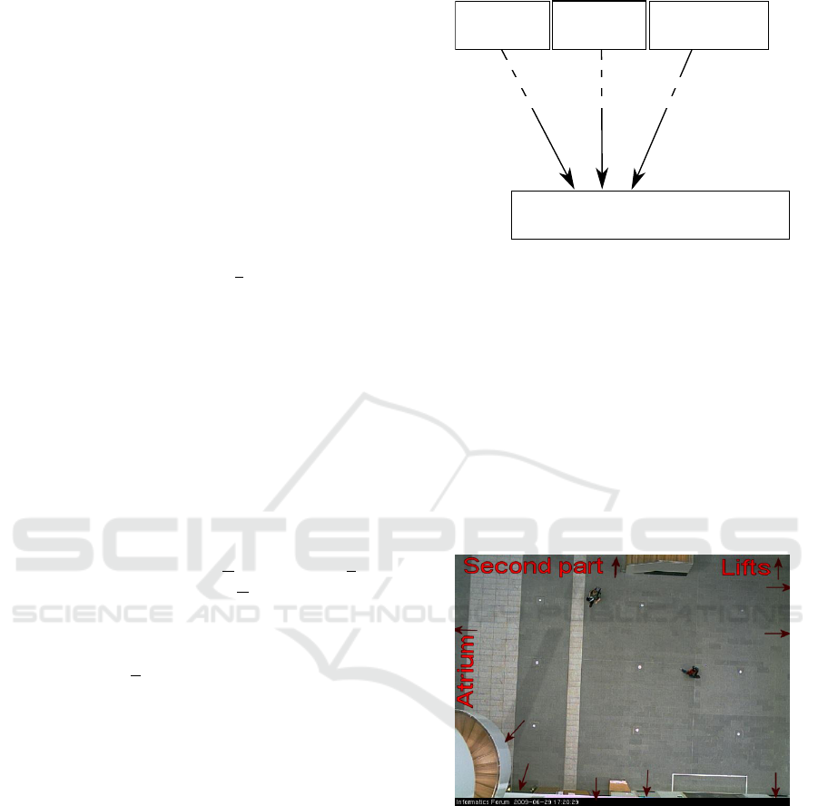
Figure 1: Overview of the proposed model.
4 EVALUATION OF THE
PREDICTION MODEL
The introduced model shall be configured for a con-
crete scenario. For this purpose, the free available
data sets from The University of Edinburgh School
of Informatics (Edinburgh Informatics Forum Pedes-
trian Database, 2010) were used as reference trajecto-
ries. The data sets consist of trajectories of people in
a forum, which were detected by a camera. In figure 2
a frame of the camera is depicted.
Figure 2: Overview of the Informatics Forum in the School
of Informatics at the University of Edinburgh. Red arrows
mark the different entrances of the forum. Original photo
from (Edinburgh Informatics Forum Pedestrian Database,
2010).
4.1 Pedestrian Scenario
In order to evaluate the efficiency of the proposed
model, the given data set was filtered by a scenario,
in which the pedestrian only has got one goal and an
obstacle in his way. Therefore, the way between the
lower right corner of the forum to the “Second part”
near the stair cases is chosen (c.f. figure 2). Only tra-
jectories of single person (no groups) are taken and it
VISAPP 2017 - International Conference on Computer Vision Theory and Applications
512

is assumed that there are not any dynamic interactions
between pedestrians. As a result of this selection, 100
trajectories are chosen, which were used for the val-
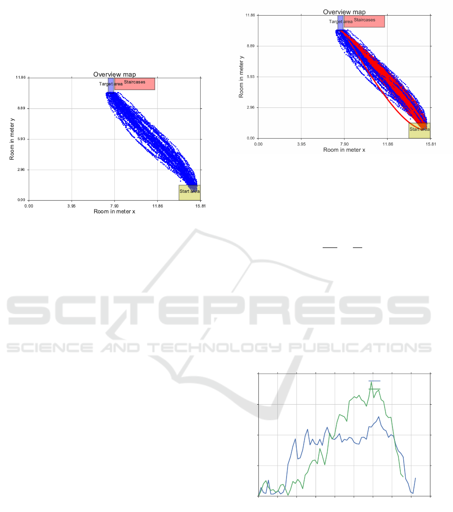
idation of the model. Figure 3 shows a plot of all
analyzed trajectories.
Figure 3: Plot of all trajectories extracted from the data set
in Informatics Forum. Every trajectory starts in the start-
ing area and ends in the target area. The staircases are ab-
stracted as a rectangular obstacle.
4.2 Experimental Results
For the initial condition k = 0, the position of the state
vector is set to the first position of the real observed
trajectory. The velocity vector is approximated by lin-
ear regression of the first ten data points of the real
observed trajectory.
Based on the prediction model, trajectories for all
selected data sets were predicted. It is obvious that
both trajectories almost match at the start. This is
due to the fact that the initial conditions are quite
the same. Other prediction steps are only calculated
based on the intention and map information, that are
the target area and the single obstacle “staircases” in
this scenario. There is no additional update nor cor-
rection of the observed trajectory. This can be inter-
preted in the way that no further measurements beside
the measurement of the initial condition are assumed.
In Figure 4 all extracted trajectories and corre-
sponding predicted trajectories are plotted. For an ob-
jective evaluation, the root mean square error (RMSE)
between the real and the observed trajectories is cal-
culated.
As the predicted trajectory is more dense than the
observed trajectory, the distance of every data point of
the observed trajectory to the nearest data point of the
predicted trajectory is calculated. The mean value of
all data points of all trajectories is calculated and de-
noted as RMSE. For 100 trajectories, D
i
data points
of the i-th observed trajectory and the minimum dis-
Figure 4: Plot of all extracted trajectories from the data set
in Informatics Forum (blue dots) and the predicted trajecto-
ries (red dots).
tance between the observed and predicted trajectory
d
i j
for the j-th data point the RMSE is given by
RMSE =
1
100
100
∑
i
1
D
i
D
i
∑
j
d
i j
(22)
In Figure 5 the course of d
i j
for two example tra-
jectories i = 20 and i = 40 is depicted. As the starting
condition of the prediction is initialized with the first
point of the observed trajectory, both trajectories have
got a difference of d
i j
= 0 for j = 0. In dependence
on the real movement of the pedestrian d
i j
rises to a
maximum of 0.3 m .. .0.6 m. The curve declines till
the end, as both curves end in the target area.
0 8 16 23 31 39 47 54 62 70
data point j of observed trajectory i
0.00
0.15
0.30
0.45
0.60
distance d
ij
Distance between observed and predicted trajectory
Trajectory i = 40
Trajectory i = 20
Figure 5: Difference between the observed and the pre-
dicted trajectory d
i j
for two example trajectories i = 20 and
i = 40.
For the given scenario a RMSE ≈ 0.29 m is ob-
tained. These are very good results. Further improve-
ments could be possible, if planning for the pedestri-
ans is assumed. In this simple scenario the behavior
of the pedestrians is only reactive to obstacles. This
means, that the pedestrian goes in the direction of the
Pedestrian Tracking using a Generalized Potential Field Approach
513

goal until he meets an obstacle and then surrounds the
obstacle in the direction of the potential gradient.
5 CONCLUSIONS
Typical mathematical models for the fusion of infor-
mation sources have got many parameters, which has
to be learned automatically by real world scenarios.
In this paper, the information sources are modeled as
potential fields accelerating a pedestrian in the field,
which minimizes the number of parameters and gives
an intuitive interpretation of them. The proposed
model is configured for a simple real world scenario.
In this scenario, two information sources, the inten-
tion and the map information, are considered. The
model is evaluated using real camera based trajec-
tories. The RMSE is calculated and shows a devia-
tion of 0.29 m between the predicted and observed
trajectory. For future research more complex scenar-
ios can be considered. These scenarios shall include
multi-hypotheses and more information sources like
dynamic pedestrian interactions and group behaviors.
REFERENCES
Alberti, E. and Belli, G. (1978). Contributions to the
boltzmann-like approach for traffic flow. a model for
concentration dependent driving programs. Trans-
portation Research, 12(1):33–42.
Ali, S. and Shah, M. (2008). Floor fields for tracking in
high density crowd scenes. In European conference
on computer vision, pages 1–14. Springer.
Bandyopadhyay, T., Jie, C. Z., Hsu, D., Ang Jr, M. H., Rus,
D., and Frazzoli, E. (2013a). Intention-aware pedes-
trian avoidance. In Experimental Robotics, pages
963–977. Springer.
Bandyopadhyay, T., Won, K. S., Frazzoli, E., Hsu, D., Lee,
W. S., and Rus, D. (2013b). Intention-aware motion
planning. In Algorithmic Foundations of Robotics X,
pages 475–491. Springer.
Dijkstra, J., Jessurun, J., and Timmermans, H. J. (2001).
A multi-agent cellular automata model of pedestrian
movement. Pedestrian and evacuation dynamics,
pages 173–181.
Dirk Helbing and Peter Molnar (1995). Social force model
for pedestrian dynamics. Phys. Rev. E, 51:4282–4286.
Edinburgh Informatics Forum Pedestrian Database (2010).
Edinburgh informatics forum pedestrian database.
http://homepages.inf.ed.ac.uk/rbf/FORUMTRACK
ING/. Accessed: 2016-10-04.
Fugger, T., Randles, B., Stein, A., Whiting, W., and Gal-
lagher, B. (2000). Analysis of pedestrian gait and
perception-reaction at signal-controlled crosswalk in-
tersections. Transportation Research Record: Journal
of the Transportation Research Board, 1(1705):20–
25.
Heinemann, P., Becker, H., and Zell, A. (2006). Improved
path planning in highly dynamic environments based
on time variant potential fields. VDI BERICHTE,
1956:177.
Helbing, D. (1998). A fluid dynamic model for the
movement of pedestrians. arXiv preprint cond-
mat/9805213.
Ibisch, A., Houben, S., Michael, M., Kesten, R., and
Schuller, F. (2015). Arbitrary object localization and
tracking via multiple-camera surveillance system em-
bedded in a parking garage. In Loce, R. P. and Saber,
E., editors, Proceedings of Spie, page 94070G.
Keller, C. G. and Gavrila, D. M. (2014). Will the Pedes-
trian Cross? A Study on Pedestrian Path Prediction.
IEEE Transactions on Intelligent Transportation Sys-
tems, 15(2):494–506.
Kretz, T. and Schreckenberg, M. (2006). FAST-floor
field-and agent-based simulation tool. arXiv preprint
physics/0609097.
Luber, M., Stork, J. A., Tipaldi, G. D., and Arras, K. O.
(2010). People tracking with human motion predic-
tions from social forces. In Robotics and Automa-
tion (ICRA), 2010 IEEE International Conference on,
pages 464–469. IEEE.
L
¨
uders, K. . O. G. (2008). Mechanik, Akustik, W
¨
arme -
Walter de Gruyter, Berlin.
Niemeier, W. (2008). Ausgleichungsrechnung - statistische
Auswertemethoden. Walter de Gruyter, Berlin, 2. aufl.
edition.
Prigogine, I. (1900). A boltzmann-like approach to the sta-
tistical theory of traffic flow. Theory of traffic flow.
Robin, T., Antonini, G., Bierlaire, M., and Cruz, J. (2009).
Specification, estimation and validation of a pedes-
trian walking behavior model. Transportation Re-
search Part B: Methodological, 43(1):36–56.
Sigloch, H. (2009). Technische Fluidmechanik -. Springer-
Verlag, Berlin Heidelberg New York, 7. aufl. edition.
Tamura, Y., Dai Le, P., Hitomi, K., Chandrasiri, N. P.,
Bando, T., Yamashita, A., and Asama, H. (2012). De-
velopment of pedestrian behavior model taking ac-
count of intention. In 2012 IEEE/RSJ International
Conference on Intelligent Robots and Systems, pages
382–387. IEEE.
Tiemann, N. (2012). Ein Beitrag zur Situationsanalyse
im vorausschauenden Fussg
¨
angerschutz. PhD thesis,
Universit
¨
at Duisburg-Essen, Fakult
¨
at f
¨
ur Ingenieur-
wissenschaften Maschinenbau und Verfahrenstechnik
Institut f
¨
ur Mechatronik und Systemdynamik.
Wakim, C. F., Capperon, S., and Oksman, J. (2004). A
Markovian model of pedestrian behavior. In Systems,
Man and Cybernetics, 2004 IEEE International Con-
ference on, volume 4, pages 4028–4033. IEEE.
Yi, S., Li, H., and Wang, X. (2015). Understanding pedes-
trian behaviors from stationary crowd groups. In Pro-
ceedings of the IEEE Conference on Computer Vision
and Pattern Recognition, pages 3488–3496.
VISAPP 2017 - International Conference on Computer Vision Theory and Applications
514