
W-PnP Method: Optimal Solution for the Weak-Perspective n-Point
Problem and Its Application to Structure from Motion
Levente Hajder
Machine Perception Research Laboratory, MTA SZTAKI,
Kende utca 13-17., H-1111 Budapest, Hungary
hajder.levente@sztaki.mta.hu
Keywords:
Weak-perspective Projection, Calibration, PnP, Structure from Motion.
Abstract:
Camera calibration is a key problem in 3D computer vision since the late 80’s. Most of the calibration methods
deal with the (perspective) pinhole camera model. This is not a simple goal: the problem is nonlinear due to
the perspectivity. The strategy of these methods is to estimate the intrinsic camera parameters first; then
the extrinsic ones are computed by the so-called PnP method. Finally, the accurate camera parameters are
obtained by slow numerical optimization. In this paper, we show that the weak-perspective camera model
can be optimally calibrated without numerical optimization if the L
2
norm is used. The solution is given by
a closed-form formula, thus the estimation is very fast. We call this method as the Weak-Perspective n-Point
(W-PnP) algorithm. Its advantage is that it simultaneously estimates the two intrinsic weak-perspective camera
parameters and the extrinsic ones. We show that the proposed calibration method can be utilized as the solution
for a subproblem of 3D reconstruction with missing data. An alternating least squares method is also defined
that optimizes the camera motion using the proposed optimal calibration method.
1 INTRODUCTION
The problem of optimal methods in multiple view ge-
ometry (Hartley and Kahl, 2007) is a very challenging
research issue. This study deals with camera calibra-
tion, a key problem in computer vision. There are
well-known solutions (Hartley and Zisserman, 2000;
Zhang, 2000) to calibrate the perspective camera;
these methods give a rough estimate of the parameters
first, then refine them using numerical optimization,
such as the Levenberg-Marquardt iteration. Optimal
camera calibrations using the L
2
norm including the
popular Perspective n-point Problem (PnP) were pub-
lished for the perspective camera only if the intrin-
sic camera parameters are known (Schweighofer and
Pinz, 2008; Lepetit et al., 2009; Hesch and Roumeli-
otis, 2011; Zheng et al., 2013). The calibration can
also be solved under the L
∞
norm (Kahl and Hart-
ley, 2008) as well as the Structure from Motion prob-
lem (Ke and Kanade, 2005; Okatani and Deguchi,
2006; Bue et al., 2012); however, the uncalibrated
problem has not been optimally solved yet in the least
squares sense to the best of our knowledge.
Weak-perspective Camera Calibration. The opti-
mal estimation of the affine calibration is easy since
it is a linear problem as it has been shown in sev-
eral studies, such as that of Shum et al. (Shum et al.,
1995). The weak-perspective (DeMenthon and Davis,
1995) and paraperspective (Horaud et al., 1997) cal-
ibration have also been considered, but the proposed
algorithms are not optimal since these papers focus on
finding the link between para/weak-perspectivity and
real projection. Kanatani et. al (Kanatani et al., 2007)
also dealt with the calibration of different affine cam-
eras, but they did not consider the optimality itself.
The scaled orthographic calibration can optimally
be calibrated as recently discussed in the work of Ha-
jder et al. (L. Hajder and
´
A. Pernek and Cs. Kaz
´
o,
2011). An iteration was proposed by the authors to
calibrate the scaled orthographic camera, and it con-
verges to the global minima as proved in (L. Hajder
and
´
A. Pernek and Cs. Kaz
´
o, 2011). The orthographic
camera is not considered separately, but the method
can be used for that purpose as well if the scale of the
scaled orthographic camera is fixed. Another possible
solution (Marques and Costeira, 2009) for the scaled
orthographic calibration is to do an affine calibration
and then find the closest scaled orthographic camera
matrix to the affine one. However, optimality cannot
be guaranteed in this case.
The optimal camera calibration method is pro-
posed for weak-perspective cameras in this paper;
Hajder L.
W-PnP Method: Optimal Solution for the Weak-Perspective n-Point Problem and Its Application to Structure from Motion.
DOI: 10.5220/0006158902650276
In Proceedings of the 12th International Joint Conference on Computer Vision, Imaging and Computer Graphics Theory and Applications (VISIGRAPP 2017), pages 265-276
ISBN: 978-989-758-227-1
Copyright
c
2017 by SCITEPRESS – Science and Technology Publications, Lda. All rights reserved
265

it estimates the camera parameters if 3D–2D point
correspondences are known between the points of a
3D calibration object and corresponding locations on
the image. The minimization is optimal in the least
squares sense.
Weak-perspective Structure from Motion. The op-
timal weak-perspective camera calibration is theoreti-
cally very interesting, and it has practical significance
as well. We show here that the calibration algorithms
can be inserted into 3D reconstruction - also called
Structure from Motion (SfM) - pipelines as a substep
yielding very efficient weak-perspective reconstruc-
tion. Mathematically, the problem is a factorization
one: the so-called measurement matrix has to be fac-
torized into the matrices containing camera and struc-
ture parameters.
The classical factorization method, when the
measurement matrix is factorized into 3D motion
and structure matrices, was developed by Tomasi
and Kanade (Tomasi, C. and Kanade, T., 1992) in
1992. The weak-perspective extension was published
by Weinshall and Kanade (Weinshall and Tomasi,
1995). Factorization was extended to the paraperspec-
tive (Poelman and Kanade, 1997) case as well as to
the real perspective (Sturm and Triggs, 1996) one.
The problem of missing data is also a very im-
portant challenge in 3D reconstruction: one cannot
guarantee that the feature points can be tracked over
the whole image sequence since feature points can
appear and/or disappear between frames. The prob-
lem of missing data was already addressed by Tomasi
and Kanade (Tomasi, C. and Kanade, T., 1992); how-
ever, they use only a naive approach which transforms
the missing data problem to the full matrix factor-
ization by estimating the missing entries. Shum et
al. (Shum et al., 1995) gave a method to reconstruct
the objects from range images; their method was suc-
cessfully applied to the SfM problem by Buchanan et
al. (Buchanan and Fitzgibbon, 2005).
The mainstream idea for factorization with miss-
ing data is to decompose the rank 4 measurement ma-
trix into affine structure and motion matrices which
are of dimension 4. The Shum-method (Shum et al.,
1995; Buchanan and Fitzgibbon, 2005) also computes
affine structure and motion matrices, but the dimen-
sion of those matrices is 3. This problem can math-
ematically be solved by Principal Component Anal-
ysis with Missing Data (PCAMD) as pointed out by
mathematicians since the middle 70’s (Ruhe, 1974).
These methods can be applied directly to the SfM
problem as it is written in (Buchanan and Fitzgibbon,
2005). Hartley & Schaffalitzky (Hartley and Schaffal-
itzky, 2003) proposed the PowerFactorization method
which is based on the Power method to compute the
dominant n-dimensional subspace of a given matrix.
Buchanan & Fitzgibbon (Buchanan and Fitzgibbon,
2005) handled the problem as an alternation consist-
ing of two nonlinear iterations to be solved; they
suggested the usage of the Damped-Newton method
with line search to compute the optimal structure and
motion matrices. Kanatani et al. (Kanatani et al.,
2007) showed that the reconstruction problem can
be solved without a full matrix factorization. Mar-
ques&Costeira (Marques and Costeira, 2009) solved
the factorization problem considering the scaled or-
thographic camera constraints; their method was ba-
sically an affine factorization, but the camera matrices
were refined based on scaled orthographic constraint
at the end of each cycle. An interesting approach was
also proposed by Whang et al. (Wang et al., 2008):
their so-called quasi-perspective reconstruction fills
the gap between affine and perspective approaches.
Contribution. The closest work to this paper is pro-
posed by Hajder et al. (L. Hajder and
´
A. Pernek and
Cs. Kaz
´
o, 2011). They proved that the scaled ortho-
graphic camera can optimally be calibrated by an it-
erative algorithm and the calibration can be applied in
the SfM approach. We deal with the weak-perspective
camera model instead of the scaled orthographic one
here. We give a closed-form solution to the cali-
bration problem, which can be inserted into iterative
SfM algorithms similarly to (L. Hajder and
´
A. Pernek
and Cs. Kaz
´
o, 2011; Kanatani et al., 2007; Marques
and Costeira, 2009) and (Buchanan and Fitzgibbon,
2005). The novelty here is that all of the steps within
the iterations are optimal. Another strength of our
method is that it can be proved that the iteration con-
verges to the closest minimum.
The optimal method proposed here is interesting
theoretically and useful practically. For the latter pur-
pose, we show that the proposed weak-perspective
factorization can give good initial values for perspec-
tive bundle adjustment (B. Triggs and P. McLauchlan
and R. Hartley and A. Fitzgibbon, 2000), and it can
be inserted into a 3D reconstruction pipeline.
The main contribution of this paper is threefold:
(i) an optimal weak-perspective calibration algorithm
(the W-PnP method) is proposed here. The optimal
solution is written in closed form given by finding the
root of a polynomial with degree 11
1
; (ii) contrary to
the standard PnP methods, the proposed calibration
algorithm estimates both the intrinsic and extrinsic
camera parameters. It is possible since the applica-
tion of the weak-perspective projection eliminates the
division from the projective equations; (iii) a weak-
1
However, the root-finding of a 11-degree polynomial
can only be carried out by numerical methods according to
the Abel-Ruffini theorem.
VISAPP 2017 - International Conference on Computer Vision Theory and Applications
266

perspective SfM algorithm is proposed here which is
an alternation with two main steps: the 3D structure
of the object to be reconstructed as well as the camera
motion are calculated optimally. The latter is done by
the proposed optimal weak-perspective camera cali-
bration method. The proposition of an alternating-
style SfM method is not novel, the main advantage
here is the application of weak-perspective projection
which makes all supsteps within the iteration optimal.
Another mentionable property of our method is that it
can cope with missing data.
Structure of Paper. In section 2, we introduce basic
notations and present formulas to write mathemati-
cally the problem. The proposed optimal camera cal-
ibration is described in section 3. Then the calibra-
tion method is inserted into an alternating-style SfM
algorithm. The proposed algorithm is tested on syn-
thesized data (section 5) as well as on coordinates
of tracked feature points from real image sequences
(section 6). Finally, the paper concludes the research
in section 7.
2 PROBLEM STATEMENT
Given the 3D coordinates of the points of a static ob-
ject and their 2D projections in the image, the aim of
camera calibration is to estimate the camera parame-
ters which represent the 3D → 2D mapping.
Let us denote the 3D coordinates of the i
th
point
by X
i
, Y
i
, and Z
i
. The corresponding 2D coordinates
are denoted by u
i
, and v
i
. The perspective (pinhole)
camera model is usually written as follows
u
i
v
i
1
∼ C[R|T
3D
]
X
i
Y
i
Z
i
1
T
. (1)
where R is the rotation (orthonormal) matrix, and T
3D
the spatial translation vector between the world and
object coordinate systems. (these parameters are usu-
ally called the extrinsic parameters of the perspective
camera) The ‘operator ∼’ denotes equality up to an
unknown scale. The intrinsic parameters of the cam-
era are stacked in the upper triangular matrix C (Hart-
ley and Zisserman, 2000).
If the above equation is multiplied by the in-
verse of camera matrix C, the following basic cam-
era calibration formula is obtained: C
−1
[u
i
v
i
1] ∼
[R|T
3D
]
X
i
Y
i
Z
i
1
T
. If the intrinsic parame-
ters stacked in matrix C and the spatial coordinates
in
X
i
Y
i
Z
i
1
T
are known then the calibra-
tion problem is reduced to the estimation of the ex-
trinsic matrix/vector R and T
3D
. This is the so-called
Perspective n-point Problem (PnP). There are several
Scaled orthographic Weak−perspective
Affine
Figure 1: Pixels for different camera models. Scaled or-
thographic, weak-perspective and affine camera pixels are
equivalent to square, rectangle, and parallelogram, respec-
tively.
efficient solvers (Schweighofer and Pinz, 2008; Lep-
etit et al., 2009; Hesch and Roumeliotis, 2011; Zheng
et al., 2013) for PnP, however, estimates for the in-
trinsic parameters of the applied cameras are usually
not presented. We deal with this problem, and it is
shown here that the weak-perspective camera calibra-
tion is possible without the knowledge of any intrinsic
camera parameters.
If the depth of object is much smaller than the dis-
tance between the camera and the object, the weak-
perspective camera model is a good approximation:
u
i
v
i
T
= [M|t]
X
i
Y
i
Z
i
1
T
. (2)
where M is the motion matrix consisting of two 3D
vectors (M = [m
1
,m
2
]
T
) and t is a 2D offset vector
which locates the position of the world’s origin in the
image.
Contrary to the affine camera model, the rows of
the motion matrix are not allowed to be arbitrary for
the weak-perspective projection, they must satisfy the
orthogonality constraint m
T
1
m
2
= 0. A special case of
the weak-perspective camera model is the scaled or-
thographic one, when m
T
1
m
1
= m
T
2
m
2
. If the affine
camera is considered, there is no constraint: the ele-
ments of the motion matrix M may be arbitrary.
The difference between the camera models can be
visualized by the shapes of the corresponding camera
pixels. Affine camera model is represented by a rect-
angular pixel: the opposite sides are parallel to each
other. The weak-perspective model constraints that
the adjacent sides are perpendicular, while the length
of the sides are equal for the scaled orthographic cam-
era model. The pixels are pictured in Fig. 1.
The optimal calibration of the affine camera in the
least squares sense is relatively simple as the projec-
tion in Eq. 2 is linear w.r.t. unknown parameters.
The solution can be obtained by the Moore-Penrose
pseudo-inverse.
The scaled orthographic camera estimation is a
more challenging problem. To the best of our knowl-
edge, there is no closed-form solution. Hajder et
al. (L. Hajder and
´
A. Pernek and Cs. Kaz
´
o, 2011)
proved that the optimal estimation can be given via
an iteration. However, their method is relatively slow
due to the iteration. The main contribution of this
paper is that the weak-perspective case is solvable
as a root finding problem of a 11-degree polyno-
mial.
W-PnP Method: Optimal Solution for the Weak-Perspective n-Point Problem and Its Application to Structure from Motion
267

3 OPTIMAL CAMERA
CALIBRATION FOR
WEAK-PERSPECTIVE
PROJECTION: THE W-PnP
METHOD
In this section, a novel weak-perspective camera cal-
ibration is proposed. The goal of the calibration is to
minimize the squared reprojection error in the least
squares sense. This is written as
1
2
N
∑
i=1
u
i
v
i
T
− [M|t]
X
i
Y
i
Z
i
1
T
2
,
(3)
where N is the number of points to be considered in
the calibration, and
||
·
||
denotes the L
2
(Euclidean)
vector norm. As Horn et al. (Horn et al., 1988)
proved, the translation vector t is optimally estimated
if it is selected as the center of gravity of the 2D
points. These are easily calculated as ˜u = 1/N
∑
N
i=1
u
i
,
and ˜v = 1/N
∑
N
i=1
v
i
.
If the weak-perspective camera model is assumed,
the error defined in eq. (3) can be rewritten in a more
compact form as
1
2
w
T
1
− m
T
1
S
2
+
1
2
w
T
2
− m
T
2
S
2
, (4)
where
w
1
= [u
1
− ˜u,u
2
− ˜u,..., u
N
− ˜u]
T
, (5)
w
2
= [v
1
− ˜v,v
2
− ˜v,. .., v
N
− ˜v]
T
, (6)
S =
X
1
X
2
... X
N
Y
1
Y
2
... Y
N
Z
1
Z
2
... Z
N
. (7)
If the Lagrange multiplier λ is introduced, the
weak-perspective constraint can be considered. The
error function is modified as follows
1
2
w
1
− m
T
1
S
2
+
1
2
w
2
− m
T
2
S
2
+ λm
T
1
m
2
(8)
The optimal solution of this error function is given
by its derivatives with respect to λ, m
1
, and m
2
:
m
T
1
m
2
= 0, (9)
SS
T
m
1
− Sw
1
+ λm
2
= 0, (10)
SS
T
m
2
− Sw
2
+ λm
1
= 0. (11)
m
2
is easily expressed from eq. (10) as
m
2
=
1
λ
Sw
1
− SS
T
m
1
. (12)
If one substitutes m
2
into eq. (11), and (9), then the
following expressions are obtained:
1
λ
SS
T
Sw
1
− SS
T
m
1
− Sw
2
+ λm
1
= 0, (13)
1
λ
m
T
1
Sw
1
− SS
T
m
1
= 0. (14)
If eq. (13) is multiplied by λ, then m
1
can be expressed
as
m
1
=
SS
T
SS
T
− λ
2
I
−1
SS
T
Sw
1
− λSw
2
(15)
where I is the 3 × 3 identity matrix. Remark that the
matrix inversion cannot be carried out if the Lagrange
multiplier λ is one of the eigenvalues of the matrix
SS
T
. If the expressed m
1
is substituted into eq. (14),
the equation from which λ should be determined is
obtained:
1
λ
A
T
(λ)B
−T
(λ)
Sw
1
− SS
T
B
−1
(λ)A(λ)
= 0 (16)
where
A(λ) = SS
T
Sw
1
− λSw
2
(17)
B(λ) = SS
T
SS
T
− λ
2
I (18)
A(λ) and B(λ) are a vector and a matrix that have ele-
ments containing polynomials of unknown variable λ.
Such kind of vectors/matrices is called vector/matrix
of polynomials in this study. The difficulty is that
matrix B(λ) should be inverted. This inversion can
be written as a fraction of two matrices. B
−1
(λ) can
write as
B
−1
(λ) =
adj
SS
T
SS
T
− λ
2
I
det(SS
T
SS
T
− λ
2
I)
(19)
where adj(.) denotes the adjoint
2
of a matrix. It is
trivial that det (B(λ)) is a polynomial of λ, while
adj(B(λ)) is a matrix of polynomials. This expres-
sion is useful since the equation can be multiplied by
the determinants of B(λ).
If one makes elementary modifications, eq. (16)
can be rewritten as
A
T
(λ)adjB
T
(λ)
detB(λ)
detB(λ)Sw
1
− SS
T
adjB(λ)A(λ)
detB(λ)
= 0.
(20)
It is also trivial that eq. (20) is true if the numer-
ator equals zero If the denominator, the determinant
of matrix B(λ) equals zero, then the problem cannot
be solved; in this case, the 3D points in S are linearly
dependent, the points in S form a plane, or a line, or
a single point instead of a real 3D object. The La-
grange multiplier λ is calculated by solving the fol-
lowing polynomial:
A
T
(λ)adjB
T
(λ)
detB(λ)Sw
1
− SS
T
adjB(λ)A(λ)
= 0.
(21)
This final polynomial is of degree 11: A(λ), and
B(λ) have terms of degree 1, and 2, respectively.
Therefore, adj(B
T
(λ))is of degree 4, while that of
2
The transpose of the adjoint is also called the matrix of
cofactors.
VISAPP 2017 - International Conference on Computer Vision Theory and Applications
268

A
T
(λ)adj(B
T
(λ)) is 5. Since the size of B(λ) is 3 × 3,
its determinant has degree 3 · 2 = 6. Other terms are
of lower degree, the degree of the final polynomial
comes to 5 + 6 = 11.
The roots of the polynomial are 11 real/complex
numbers, but only the real values have to be consid-
ered. The obtained real values of λ should be sub-
stituted into eq. (15) and the obtained m
1
and λ into
eq. (12); then the optimal solution is the one minimiz-
ing the reprojection error given in eq. (3).
We use Joe Huwaldt’s Java Matrix Tool
3
to solve
the 11-th order polynomial equation. Our implemen-
tation uses the Jenkins and Traub root finder (Jenkins
and Traub, 1970), and we found that this algorithm is
numerically very stable.
A very important remark is that in the case, when
the coordinates in vectors w
1
and w
2
are noise-free, it
is possible that λ equals zero. Then the camera vec-
tors m
1
and m
2
can be computed as m
1
=
SS
T
−1
Sw
1
and m
2
=
SS
T
−1
Sw
1
.
Minimal Solution. For PnP algorithms, the mini-
mal number of points for the algorithms is also an
important issue. The proposed optimization method
is based on reprojection error: each point adds two
equations to the minimization. The camera matrix
consists of eight elements: six for camera pose and
scales, two for offset. The pose gives 3 Degrees of
Freedom (DoFs), vertical and horizontal scales are
two DoFs, while the offset yields another two param-
eters. In summary, the problem has 7 DoFs and they
can be estimated from at least four 3D → 2D point
correspondences.
4 STRUCTURE FROM MOTION
WITH MISSING DATA
We describe here how the previously discussed opti-
mal calibration method can be applied for the factor-
ization (SfM) problem. Our method allows the points
to appear and/or disappear; thus, it can handle the
missing data problem.
The proposed reconstruction method is an alter-
nating least squares algorithm to minimize the repro-
jection error defined as follows
H
W − [M|t]
S
1
T
2
F
, (22)
where M is the motion matrix consisting of the cam-
era parameters in every frame, and structure matrix S
3
Available at http://thehuwaldtfamily.org/java/Packages/
MathTools/MathTools.html
contains the 3D coordinates of the points (points are
located in the columns of matrix S). Operator ‘’ de-
notes the so-called Hadamard product
4
, and H is the
mask matrix. If H
i j
is zero, then the j
th
point in the
i
th
frame is not visible. If H
i j
= 1, the point is visible.
Each cycle of the proposed methods is divided
into the following main steps:
1. W-PnP-step. The aim of this step is to
optimally estimate the motion matrix M =
[M
T
1
,M
T
2
,.. ., M
T
F
]
T
, and translation vector t =
[t
T
1
,t
T
2
,.. .,t
T
F
]
T
if S is fixed, where the index de-
notes the frame number. It is trivial that the esti-
mation of these submatrices are independent from
each other if the elements of the structure matrix S
are fixed. The optimal solution is given by W-PnP
method defined in Section 3. Note that missing
data should be skipped in the estimation.
2. S-step. The goal of S-step is to compute the
structure matrix S if the elements of the mo-
tion matrix and the translation vector are fixed
5
.
The 3D points represented by the columns of the
structure matrix must be computed independently
(they are independent from each other). Missing
data should be considered during the estimation
of course. It is a linear problem w.r.t. the coor-
dinates contained by structure matrix S; the op-
timal method can be obtained using the Moore-
Penrose pseudo-inverse as described in (Shum
et al., 1995).
The proposed algorithm iterates the two steps un-
til convergence as overviewed in Alg. 1. The conver-
gence itself is guaranteed since both steps decrease
the non-negative reprojection error defined in Eq 22.
The proposed factorization method requires initial
Algorithm 1: Summary of weak-perspective factorization.
M
(0)
,t
(0)
,S
(0)
← Parameter Initialization
k ← 0
repeat
k ← k + 1
M
(k)
,t
(k)
← W-PnP-Step(H,W ,S
(k−1)
)
S
(k)
← S-Step(H,W ,M
(k)
,t
(k)
)
until convergence.
values of the matrices. The key idea for initializing
the parameters is that the factorization with missing
data can be divided into full matrix factorization of
4
A B = C if c
i j
= a
i j
· b
i j
.
5
This task is usually called triangulation. This term
comes from stereo vision where the camera centers and the
3D position of the point form a triangle.
W-PnP Method: Optimal Solution for the Weak-Perspective n-Point Problem and Its Application to Structure from Motion
269

submatrices. If there is overlapping between subma-
trices, then the computed motion and structure sub-
matrices can be merged if they are rotated and trans-
lated with the appropriate rotation matrices and vec-
tors, respectively. We use the method of Pernek et
al. (Pernek et al., 2008) for this purpose.
Algorithm 2: Skeleton of Scaled Orthographic Camera Cal-
ibration.
repeat
w
3
← Completion(R,t,S,scale)
R,t,scale ← Registration(S,w
1
,w
2
,w
3
)
until convergence.
Comparison with Scaled Orthographic Factoriza-
tion. The scaled orthographic camera calibration (L.
Hajder and
´
A. Pernek and Cs. Kaz
´
o, 2011) is
overviewed in Alg 2. The main idea of the calibra-
tion is as follows: the measured 2D coordinates are
completed with a third coordinate that is simply cal-
culated by reprojecting the spatial coordinates with
the current camera parameters. Then the registration-
step refines the camera parameters, and the comple-
tion and registration steps are repeated until conver-
gence. Hajder et al. (L. Hajder and
´
A. Pernek and Cs.
Kaz
´
o, 2011) proved that this iteration converges to the
global optimum and this convergence is independent
of the initial values of the camera parameters. The
completion is simple, easy to implement, however, it
is very costly as the calibration algorithm is iterative,
closed-form solution is not known.
An alternating-style SfM algorithm can also be
formed using the scaled orthographic camera model
as it is visualized in Alg 3. It has more steps than the
weak-perspective SfM method (Alg. 1) as the com-
pletion of the 2D coordinates is required after every
other steps.
Comparison with Affine Factorization. As it is dis-
cussed before, the estimation of affine camera param-
eters is a linear problem. There are several meth-
ods (Shum et al., 1995; Buchanan and Fitzgibbon,
2005) dealing with affine SfM factorization as well.
They are relatively fast, but the accuracy of those is
lower compared to the scaled orthographic and weak-
perspective factorization as the affine camera model
enables shearing (skew) of the images that is not a
realistic assumption. Remark that the skeleton of
the affine SfM methods is the same as that of weak-
perspective one defined in Alg. 1.
Source Code. The proposed weak-perspective SfM
algorithm is implemented in Java and will be available
after publication.
Algorithm 3: Summary of scaled orthographic factoriza-
tion.
M
(0)
,t
(0)
,S
(0)
← Parameter Initialization
˜
H,
˜
W
(0)
,
˜
M
(0)
,
˜
t
(0)
← Complete(H, W ,M
(0)
,t
(0)
,
S
(0)
)
k ← 0
repeat
k ← k + 1
˜
M
(k)
← Registration(
˜
H,
˜
W
(k)
,S
(k−1)
)
˜
W
(k)
← Completion(W,
˜
H,
˜
M
(k)
,S
(k−1)
)
S
(k)
← S-Step(
˜
H,
˜
W
(k)
,
˜
M
(k)
)
˜
W
(k)
← Completion(W,
˜
H,
˜
M
(k)
,S
(k)
)
until
˜
H
˜
W
(k)
−
h
˜
M
(k)
|t
(k)
i
S
(k)
1
2
F
con-
verges.
5 TESTS ON SYNTHESIZED
DATA
Several experiments with synthetic data were carried
out to study the properties of the proposed meth-
ods. Three methods were compared: (i) SO Scaled
Orthographic factorization (L. Hajder and
´
A. Pernek
and Cs. Kaz
´
o, 2011), (ii) WP proposed Weak-
Perspective factorization, and (iii) AFF: Affine fac-
torization (Shum et al., 1995).
We have examined three properties as follows.
1. Reconstruction error: The reconstructed 3D
points are registered to the generated (ground
truth) ones using the method of Arun et al.(Arun
et al., 1987). This registration error is called
reconstruction error in the tests. The charts
show the improvement of the method (in percent-
age) w.r.t. the original Tomasi-Kanade factoriza-
tion (Tomasi, C. and Kanade, T., 1992).
2. Motion error: The row vectors of the obtained 3D
motion matrix can be registered to that of the gen-
erated (ground truth) motion matrix. This reg-
istration error is called motion error here. The
charts show the improvement in percentage sim-
ilarly to visualization of the reconstruction error.
3. Time demand: The running time of each algo-
rithm was measured. The given values contain
every step from the parameter initialization to the
final reconstruction.
To compare the affine method (Shum et al., 1995)
listed above with the other two rival algorithms, the
computation of the metric 3D structure was car-
ried out by the classical weak-perspective Tomasi-
Kanade factorization (Tomasi, C. and Kanade, T.,
1992). The 2F × 4 affine motion was multiplied by
VISAPP 2017 - International Conference on Computer Vision Theory and Applications
270

the 4 × P affine structure matrix, and a full measure-
ment matrix was obtained. Then this measurement
matrix was factorized by the Tomasi-Kanade algo-
rithm (Tomasi, C. and Kanade, T., 1992) with the
Weinshall-Kanade (Weinshall and Tomasi, 1995) ex-
tension.
All of the rival methods were implemented in
Java. The tests were run on an Intel Core4Quad 2.33
GHz PC with 4 GByte memory.
5.1 Test Data Generation
Generation of Moving Feature Points. The input
measurement matrix was composed of 2D trajecto-
ries. These trajectories were generated in the fol-
lowing way: (i) Random three-dimensional coordi-
nates were generated by a zero-mean Gaussian ran-
dom number generator with variance σ
3D
. (ii) The
generated 3D points were rotated by random angles.
(iii) Points were projected using perspective projec-
tion.
6
(iv) Noise was added to the projected coordi-
nates. It was generated by a zero-mean Gaussian ran-
dom number generator as well; its variance was set
to σ
2D
. (v) Finally, the measurement matrix W was
composed of the projected points. (vi) Motion and
structure parameters were initialized as described in
Sec. 4. For each test case, 100 measurement matrices
were generated and the results shown in this section
were calculated as the average of the 100 independent
executions.
Generation of Mask Matrix. The mask generator
algorithm has three parameters: (i) P: Number of
the visible points in each frame, (ii) F: Number of
the frames. (iii) O: offset between two neighboring
frames. The structure of the mask matrix is seen in
Fig. 2. Each point appears and disappears only once.
If a point has already disappeared it will not be visible
again in the sequence.
5.2 Test Evaluation
General Remarks. The charts basically show that
the SO algorithm outperforms the other methods in
every test case as it is expected. This is evident since
the scaled orthographic projection model is the closest
one to real perspectivity. This is true for the recon-
struction error as well as the motion error. The sec-
ond place in accuracy is given to the proposed weak-
perspective (WP) method which is always better than
6
We tried the orthographic projection model
with/without scale as well, the results had similar
characteristics. Only the fully perspective test generation is
contained in this paper due to the page limit.
0
0
1
1
F
P
o
o
o
o
.
.
.
P
P
P
Figure 2: Structure of mask matrix. Vertical and horizontal
directions correspond to the frames and points, respectively.
If an element is zero then the corresponding feature is not
visible in the pointed frames. This type of mask matrices
simulates the realistic case when the features appear and
disappear only once.
the affine one, but slightly less accurate than the SO
method.
Examining the charts of time demand, it is clear
that the fastest method is the affine (AFF) one;
however, the affine algorithm can be very slow as
discussed during real tests later if there is a huge
amount of input data. It is because a full factor-
ization (Tomasi, C. and Kanade, T., 1992) must be
applied after the affine factorization to obtain met-
ric reconstruction, and this can be very slow due
to the Singular Value Decomposition. This SVD-
step can be faster if only the three most dominant
singular values and vectors are computed (Kanatani
et al., 2007). Unfortunately, the Java Matrix Package
(JAMA) which we used in our implementation does
not contain this feature. As shown in (Buchanan and
Fitzgibbon, 2005), there are several methods which
implement affine reconstruction. Pernek et al. have
shown earlier (Pernek et al., 2008) that the fastest
method of those is the so-called Damped-Newton al-
gorithm, which is significantly faster than our affine
implementation.
The main conclusion of the tests is that there is
a tradeoff between accuracy and time demand. The
SO factorization is the most accurate but slowest one,
while the affine is fast but less accurate. The proposed
WP-SfM algorithm is very close to SO and AFF al-
gorithms in accuracy and running time, respectively.
Error Versus Noise (Figure 3). The methods were
run with gradually increasing noise level. The re-
construction error increases approximately in a linear
way for all the methods. Therefore, the improvement
is approximately the same for all noise levels as the
error of the reference factorization (Tomasi, C. and
Kanade, T., 1992) increases with regard to noise as
well. The test sequence consisted of 20 frames, and
P = 100 was set. The missing data ratio was 30.6%.
The noise level was calculated as 100σ
2D
/σ
3D
.
The test indicated that the SO algorithm outpow-
ered the rival ones, and the WP method was better
W-PnP Method: Optimal Solution for the Weak-Perspective n-Point Problem and Its Application to Structure from Motion
271
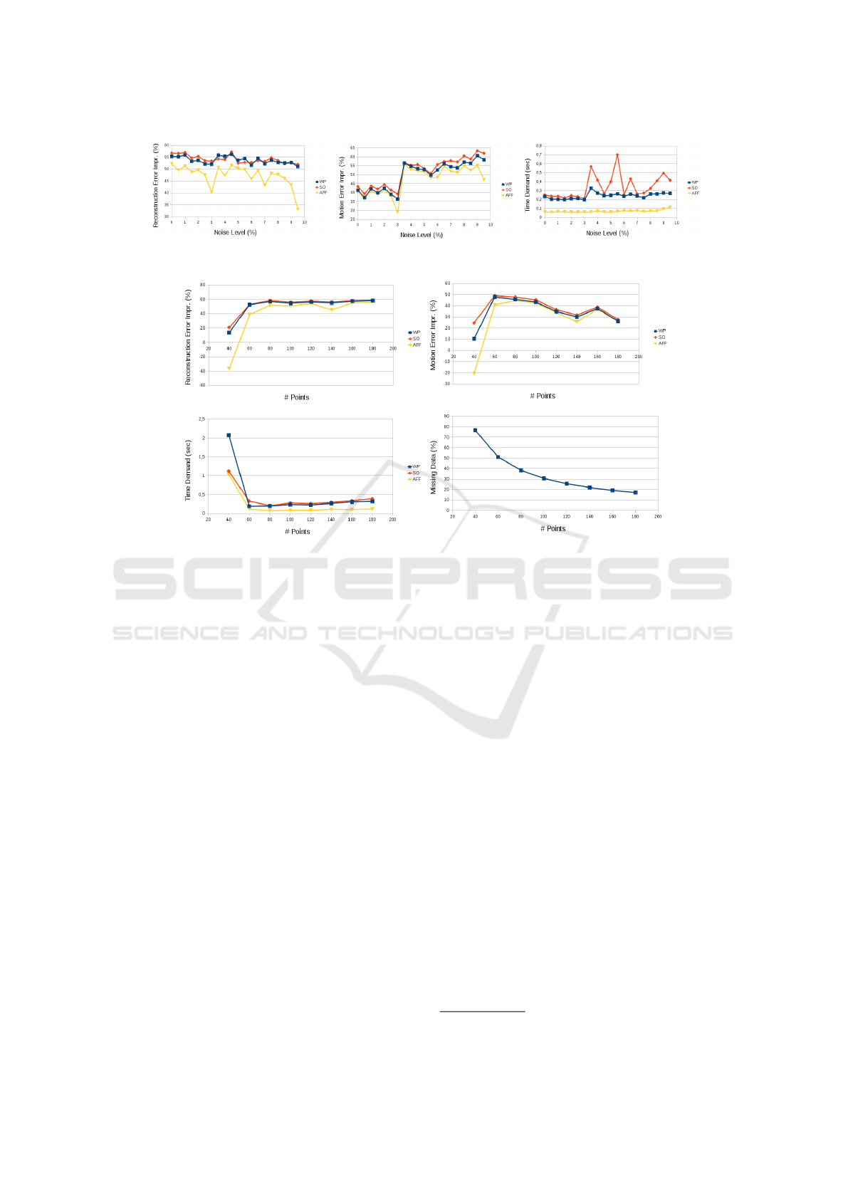
Figure 3: Improvement of reconstruction and motion errors (left charts) and time demand (right) w.r.t. 2D noise.
Figure 4: Improvement of reconstruction and motion errors (top charts) and time demand (bottom left) w.r.t. number of points.
Bottom right chart shows the ratio of missing data.
than the affine one as expected; however, SO needs
the most time to finish its execution, thus the fastest
method is the affine one.
Error Versus Number of Points (Figure 4). P in-
creased from 40 to 180 (the missing data rate de-
creased from approx. 80% to 20%). The noise level
was 5%, and the sequence consisted of 100 frames.
The conclusion was similar to the previous test case:
the most accurate model was given by the SO algo-
rithm, the second one was from the WP method. The
difference was not significant in either accuracy or ex-
ecution time.
Error Versus Number of Frames (Figure 5). F
increased from 10 to 46. The corresponding miss-
ing data ratio increased from 10% to 80%.The noise
level was 5%, and P = 100. In each test case, the
most accurate algorithm was the one consisting of
the scaled orthographic camera model, but this was
also the slowest one as expected. The accuracy of the
weak-perspective factorization is better than the affine
one after both structure and motion reconstruction.
5.3 Parameter Initialization for Bundle
Adjustment
As discussed above, the affine, weak-perspective and
scaled orthographic SfM method can estimate the 3D
structure of the tracked points. In this chapter, we
are examining how obtained 3D points can be used
as initial parameters for perspective reconstruction.
The 3D coordinates are perspectively projected. The
applied perspective reconstruction itself is the SBA
implementation
7
of the well-known bundle adjust-
ment (B. Triggs and P. McLauchlan and R. Hartley
and A. Fitzgibbon, 2000) method.
When the structure matrices have already been
computed, the estimation of the 3 × 4 projection ma-
trices is a camera calibration problem. In our test, the
normalized Direct Linear Transformation (DLT) algo-
rithm (Hartley and Zisserman, 2000) was applied (it
is also known as the ’six-point method’). The projec-
tion matrix was then decomposed into camera intrin-
sic and extrinsic parameters.
We compared the initial parameters of the three
compared method. BA cannot guarantee that global
optimum is reached through estimation; it is inter-
7
http://users.ics.forth.gr/∼lourakis/sba/
VISAPP 2017 - International Conference on Computer Vision Theory and Applications
272
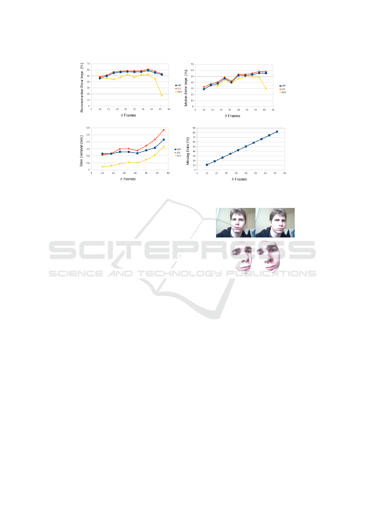
Figure 5: Improvement of reconstruction and motion errors (top charts) and time demand (bottom left) w.r.t. number of
frames. Bottom right chart show the ratio of missing data.
esting that BA after the weak-perspective, scaled or-
thographic and affine parameter initialization usually
gives the same results. The time demand of the two
methods differs a bit: the weak-perspective (WP) and
scaled orthographic (SO) methods usually help BA to
yield faster convergence than affine (AFF) parameter-
ization. We also applied the classical Tomasi-Kanade
(TK) algorithm (Tomasi, C. and Kanade, T., 1992) for
parameter initialization, and that yielded the slowest
BA convergence. Moreover, its results were usually
less accurate than those of the other three algorithms
(AFF,SO,WP); therefore, it seems that BA usually
converges to local minima if the initial parameters are
obtained by Tomasi-Kanade factorization. Time de-
mand (msec) in our test sequences are listed in Ta-
ble 1. There is not significant difference between the
case when the scaled orthographic or proposed weak-
perspective factorization is applied in order to com-
pute initial parameters for perspective BA. Therefore
the overall running time of WP method is smaller as
the WP factorization is faster than the SO one.
The conclusion of the parameter initialization
test is that the weak-perspective algorithm gives the
fastest results since the time demand for factorization
itself is faster than that of rival methods, while the
speed of the BA algorithm is approximately the same
in the case of WP and SO parameter initialization; the
BA method usually converges to the same 3D recon-
structions.
Figure 6: 2 out of 331 original image (top) and two views
(bottom) of the reconstructed 3D model of ’Face’ sequence.
6 TESTS ON REAL DATA
We tested the proposed algorithm on several real se-
quences.
’Face’ Sequence. Our first test sequence consisted of
331 images of a quasi-rigid human face as visualized
in the left two plots of Fig. 6. We computed a two-
dimensional Active Appearance Model (Matthews
and Baker, 2003) (AAM) that contained 44 feature
points of the face. The tracking was done by a mod-
ified implementation of GreatYao library. The miss-
ing ratio in this example is 0% since the AAM model
computation estimates all the points in all the frames.
The proposed weak-perspective algorithm success-
fully computed the 3D coordinates of the AAM fea-
ture points as pictured in the right part of Fig. 6
(the points are triangulated and the whole model is
textured based on one of the original image). We
tried the scaled orthographic reconstruction method
W-PnP Method: Optimal Solution for the Weak-Perspective n-Point Problem and Its Application to Structure from Motion
273
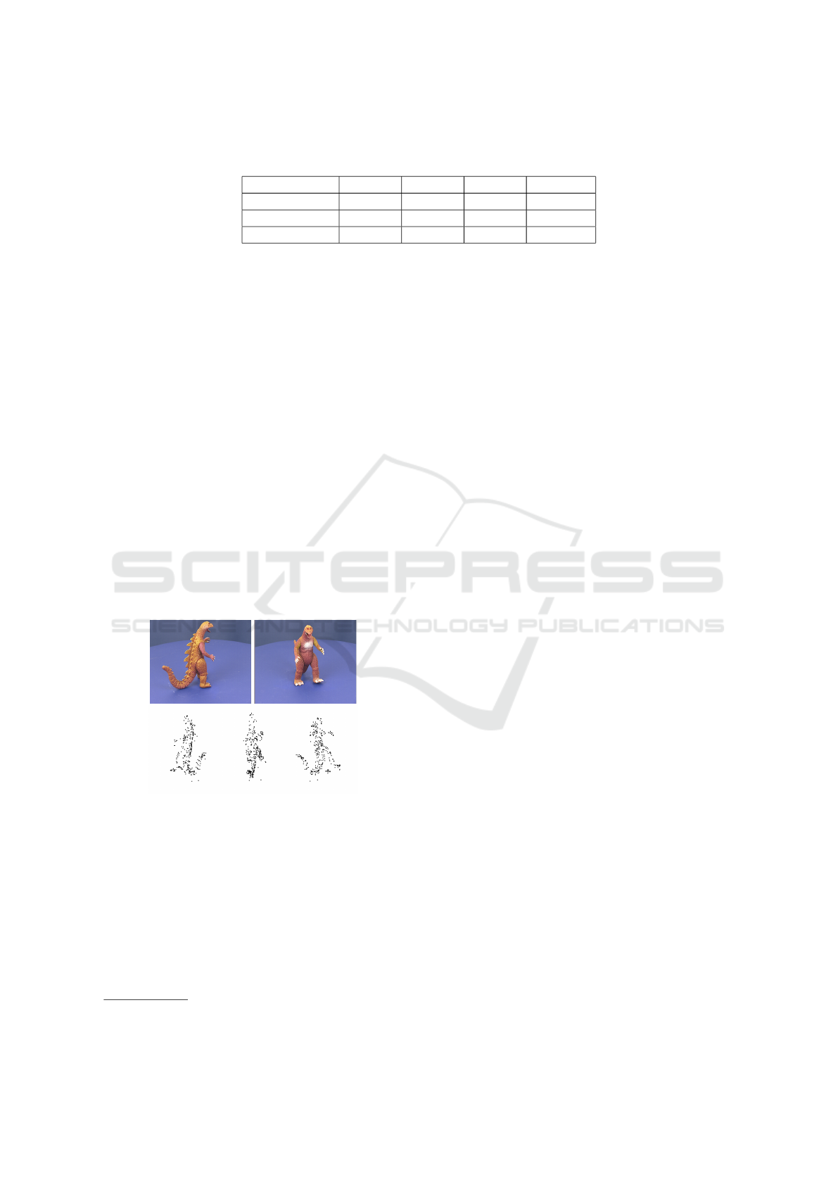
Table 1: Time demand of Bundle Adjustment. There is not significant difference between the scaled orthographic (SO) and
weak-perspective (WP) values.
Test Sequence TK WP SO Aff
versus noise 1628.35 986.12 989.805 1033.27
versus frames 1649.63 598.93 582.22 693.77
versus points 985.65 452.525 444.7 450.4375
as well, but the affine model was not run, because
there are no missing elements in the data, thus the
classical Tomasi-Kanade factorization (Tomasi, C.
and Kanade, T., 1992; Weinshall and Tomasi, 1995)
can be carried out. The threshold ε of the stop-
ping criterion was set to 10
−5
for both the scaled or-
thographic, and the weak-perspective methods. The
time demand of the proposed algorithms was 35 secs,
while the scaled orthographic one finished its compu-
tation in 49 secs.
’Dino’ Sequence. The ’Dino’ sequence, downloaded
from the web page of the Oxford University
8
, con-
sisted of 36 frames and 319 tracked points. The mea-
surement matrix had a missing data ratio of 77%. In-
put images are visualized on the left images of Fig. 7.
The reconstructed 3D points were computed by the
proposed SfM method. The time demands of that was
26 seconds (the affine and scaled orthographic SfM
methods have computed the reconstruction in 6 and
34 seconds, respectively). The results are plotted in
the right part of Fig. 7.
Figure 7: Results on ’Dino’ sequence: Top: 2 out of 36 orig-
inal image and (bottom) reconstructed point cloud captured
from three views.
Another interesting examination is to compare the
quality of the reconstructed 3D models; the points
themselves seem very similar, but the camera posi-
tions differs significantly. We compared those after
factorization by the original Tomasi-Kanade method
to affine, weak-perspective and scaled orthographic
improvement as visualized in Fig. 8. The qual-
ity of the original factorization method (top-left im-
8
http://www.robots.ox.ac.uk/∼amb/
age) is very erroneous since the cameras should be
located at regular locations of a circle. The im-
provements are significantly better. As expected,
the scaled orthographic reconstruction (bottom-right
image) serves better quality, the proposed weak-
perspective (bottom-left) is slightly worse, but it
serves acceptable results; the affine refinement (top-
right plot) is also satisfactory.
The visualization of the camera optical centers for
non-perspective cameras was not trivial. The pose of
the cameras were obtained by the factorizations, but
the focal length could not be estimated. For this rea-
son, the focal length was set manually.
’Cat’ Sequence. We tested the proposed algorithm on
our ‘Cat’ sequence. The cat statuette was rotated on
a table and 92 photos were taken by a common com-
mercial digital camera. The regions of the statuette in
the images were automatically determined.
Feature points were detected using the widely-
used KLT (Tomasi, C. and Shi, J., 1994) algorithm,
and the points were tracked by a correlation-based
template matching method. A features point was la-
beled as missing if the tracker could not find its lo-
cation in the next image, or the location was not in-
side the automatically detected region of the object.
The measurement matrix of the sequence consisted of
2290 points and 92 frames. The missing data ratio
was 82%, that is very high.
The 3D reconstructed points are visualized on the
right plots of Fig. 9. We tested every possible method
and compared the time demand of the methods: the
running times of the affine, scaled orthographic, and
weak-perspective factorization were 484, 199, and 99
seconds, respectively.
7 CONCLUSION
We have presented the optimal calibration algorithm
for the weak-perspective camera model here. The
proposed method minimizes the reprojection error of
feature points in the least squares sense. The solu-
tion is given by a closed-form formula. We have
also proposed a SfM algorithm; it is an iterative one,
and every iteration consists of two optimal steps: (i)
The structure matrix computation is a linear problem,
VISAPP 2017 - International Conference on Computer Vision Theory and Applications
274
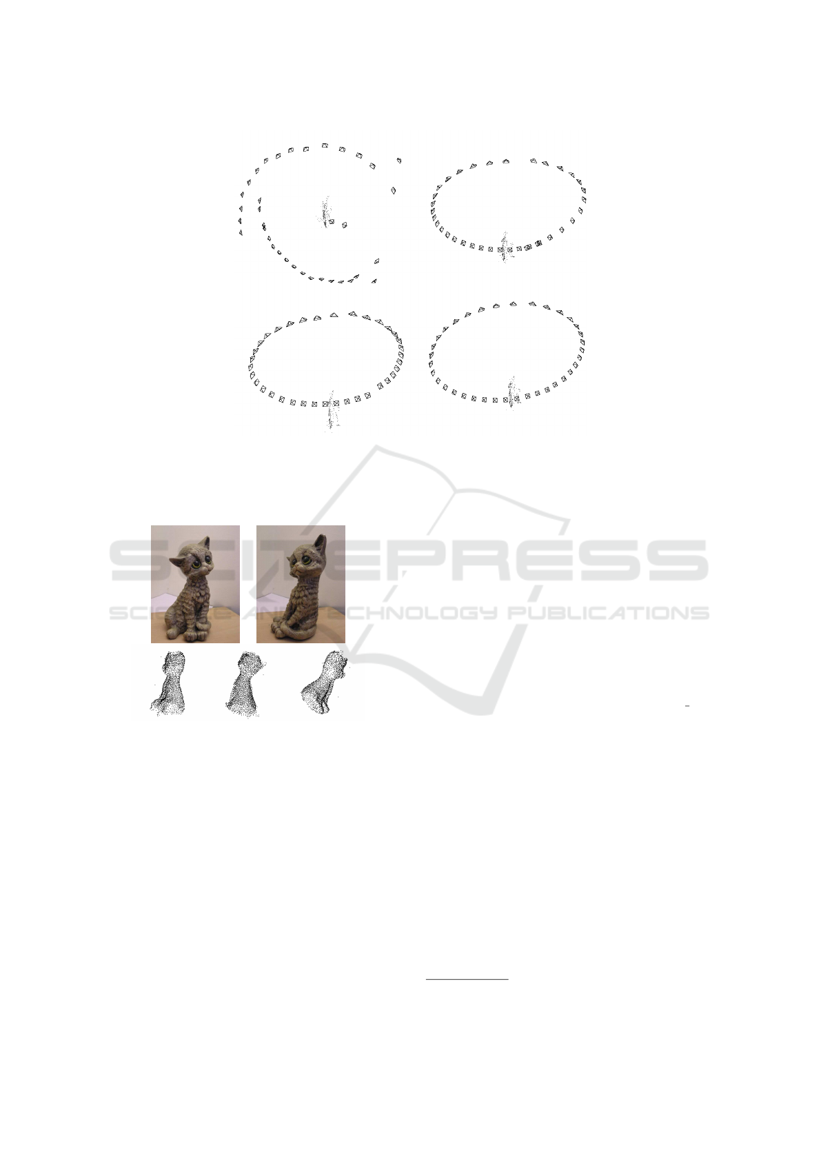
Figure 8: Reconstructed ’Dino’ model with estimated cameras. Top-left: Original Tomasi-Kanade factorization. Top-right:
Affine factorization. Bottom-left: Weak-perspective factorization (proposed method). Bottom-right: Scaled orthographic fac-
torization. The cameras should be uniformly located around the estimated point cloud of the plastic dinosaur. The difference
between weak-perspective and scaled orthographic camera parameters is not significant.
Figure 9: Two images (top) of sequence ’Cat’ and the re-
constructed points from three views (bottom).
therefore it can be optimally estimated in the least
squares sense, while (ii) the camera parameters are
obtained by the novel optimal weak-perspective cam-
era calibration method. The introduced SfM approach
can also cope with the problem of missing feature
points.
The proposed SfM algorithm was compared to the
affine (Shum et al., 1995) and scaled orthographic (L.
Hajder and
´
A. Pernek and Cs. Kaz
´
o, 2011) methods.
It was shown that our method is significantly more
accurate than the affine one, and usually faster than
the scaled orthographic SfM algorithm due to the op-
timal weak-perspective calibration. We successfully
applied the novel method to compute the initial pa-
rameters for bundle adjustment-type 3D perspective
reconstruction.
The Java implementation of our weak-perspective
SfM algorithm can be downloaded from the web
9
.
ACKNOWLEDGEMENT
This work was supported in part by the project
SCOPIA Development of software supported clinical
devices based on endoscope technology (VKSZ 14-1-
2015-0072) financed by the Hungarian National Re-
search, Development and Innovation Fund (NKFIA).
REFERENCES
Arun, K. S., Huang, T. S., and Blostein, S. D. (1987). Least-
squares fitting of two 3-D point sets. IEEE Trans. on
PAMI, 9(5):698–700.
B. Triggs and P. McLauchlan and R. Hartley and A. Fitzgib-
bon (2000). Bundle Adjustment – A Modern Synthe-
sis. In Vision Algorithms: Theory and Practice, pages
298–375.
Buchanan, A. M. and Fitzgibbon, A. W. (2005). Damped
newton algorithms for matrix factorization with miss-
ing data. In Proceedings of the 2005 IEEE CVPR,
pages 316–322.
9
http://web.eee.sztaki.hu/Factorization.zip
W-PnP Method: Optimal Solution for the Weak-Perspective n-Point Problem and Its Application to Structure from Motion
275

Bue, A. D., Xavier, J., Agapito, L., and Paladini, M. (2012).
Bilinear modeling via augmented lagrange multipliers
(balm). IEEE Trans. on PAMI, 34(8):1496–1508.
DeMenthon, D. F. and Davis, L. S. (1995). Model-based
object pose in 25 lines of code. IJCV, 15:123–141.
Hartley, R. and Kahl, F. (2007). Optimal algorithms in mul-
tiview geometry. In Proceedings of the Asian Conf.
Computer Vision, pages 13–34.
Hartley, R. and Schaffalitzky, F. (2003). Powerfactorization:
3d reconstruction with missing or uncertain data.
Hartley, R. I. and Zisserman, A. (2000). Multiple View Ge-
ometry in Computer Vision. Cambridge University
Press.
Hesch, J. A. and Roumeliotis, S. I. (2011). A direct least-
squares (dls) method for pnp. In International Con-
ference on Computer Vision, pages 383–390. IEEE.
Horaud, R., Dornaika, F., Lamiroy, B., and Christy, S.
(1997). Object pose: The link between weak per-
spective, paraperspective and full perspective. Inter-
national Journal of Computer Vision, 22(2):173–189.
Horn, B., Hilden, H., and Negahdaripourt, S. (1988).
Closed-form Solution of Absolute Orientation Using
Orthonormal Matrices. Journal of the Optical Society
of America, 5(7):1127–1135.
Jenkins, M. A. and Traub, J. F. (1970). A Three-Stage
Variables-Shift Iteration for Polynomial Zeros and Its
Relation to Generalized Rayleigh Iteration. Numer.
Math, 14:252263.
Kahl, F. and Hartley, R. I. (2008). Multiple-view geometry
under the linfinity-norm. IEEE Trans. Pattern Anal.
Mach. Intell., 30(9):1603–1617.
Kanatani, K., Sugaya, Y., and Ackermann, H. (2007).
Uncalibrated factorization using a variable symmet-
ric affine camera. IEICE - Trans. Inf. Syst., E90-
D(5):851–858.
Ke, Q. and Kanade, T. (2005). Quasiconvex Optimization
for Robust Geometric Reconstruction. In ICCV ’05:
Proceedings of the Tenth IEEE International Confer-
ence on Computer Vision, pages 986–993.
L. Hajder and
´
A. Pernek and Cs. Kaz
´
o (2011). Weak-
Perspective Structure from Motion by Fast Alterna-
tion. The Visual Computer, 27(5):387–399.
Lepetit, V., F.Moreno-Noguer, and P.Fua (2009). Epnp: An
accurate o(n) solution to the pnp problem. Interna-
tional Journal of Computer Vision, 81(2):155–166.
Marques, M. and Costeira, J. (2009). Estimating 3d shape
from degenerate sequences with missing data. CVIU,
113(2):261–272.
Matthews, I. and Baker, S. (2003). Active appearance mod-
els revisited. International Journal of Computer Vi-
sion, 60:135–164.
Okatani, T. and Deguchi, K. (2006). On the wiberg algo-
rithm for matrix factorization in the presence of miss-
ing components. IJCV, 72(3):329–337.
Pernek, A., Hajder, L., and Kaz
´
o, C. (2008). Metric Recon-
struction with Missing Data under Weak-Perspective.
In BMVC, pages 109–116.
Poelman, C. J. and Kanade, T. (1997). A Paraperspective
Factorization Method for Shape and Motion Recov-
ery. IEEE Trans. on PAMI, 19(3):312–322.
Ruhe, A. (1974). Numerical computation of principal com-
ponents when several observations are missing. Tech-
nical report, Umea Univesity, Sweden.
Schweighofer, G. and Pinz, A. (2008). Globally optimal
o(n) solution to the pnp problem for general camera
models. In BMVC.
Shum, H.-Y., Ikeuchi, K., and Reddy, R. (1995). Principal
component analysis with missing data and its appli-
cation to polyhedral object modeling. IEEE Trans.
Pattern Anal. Mach. Intell., 17(9):854–867.
Sturm, P. and Triggs, B. (1996). A Factorization Based Al-
gorithm for Multi-Image Projective Structure and Mo-
tion. In ECCV, volume 2, pages 709–720.
Tomasi, C. and Kanade, T. (1992). Shape and Motion from
Image Streams under orthography: A factorization ap-
proach. Intl. Journal Computer Vision, 9:137–154.
Tomasi, C. and Shi, J. (1994). Good Features to Track. In
IEEE Conf. Computer Vision and Pattern Recognition,
pages 593–600.
Wang, G., Wu, Q. M. J., and Sun, G. (2008). Quasi-
perspective projection with applications to 3d factor-
ization from uncalibrated image sequences. In CVPR.
Weinshall, D. and Tomasi, C. (1995). Linear and Incremen-
tal Acquisition of Invariant Shape Models From Image
Sequences. IEEE Trans. on PAMI, 17(5):512–517.
Zhang, Z. (2000). A flexible new technique for camera cal-
ibration. IEEE Trans. on PAMI, 22(11):1330–1334.
Zheng, Y., Kuang, Y., Sugimoto, S.,
˚
Astr
¨
om, K., and Oku-
tomi, M. (2013). Revisiting the pnp problem: A fast,
general and optimal solution. In ICCV, pages 2344–
2351.
VISAPP 2017 - International Conference on Computer Vision Theory and Applications
276
