Particle Convergence Expected Time in The PSO Model with Inertia

Weight

Krzysztof Trojanowski and Tomasz Kulpa

Cardinal Stefan Wyszy

nski University, Faculty of Mathematics and Natural Sciences, Warsaw, Poland

Keywords:

Particle Swarm with Inertia Weight, Particle Location Convergence Expected Time, Location Variance

Convergence Expected Time.

Abstract:

Theoretical properties of particle swarm optimization approach with inertia weight are investigated. Particu-

larly, we focus on the convergence analysis of the expected value of the particle location and the variance of

the location. Four new measures of the expected particle convergence time are deﬁned: (1) convergence of the

expected location of the particle, (2) the particle location variance convergence and (3-4) their respective weak

versions. For the ﬁrst measure an explicit formula of its upper bound is also given. For the weak versions of

the measures graphs of recorded values are presented.

1 INTRODUCTION

Particle swarm optimization (PSO) is a stochastic

population-based search algorithm successfully ap-

plied in numerous real-world problems (Poli, 2008a;

Bonyadi and Michalewicz, 2016b). Usually, when

PSO is implemented some drawbacks or limitations

can be observed. They can be divided into two

main groups: related to transformation invariance and

to convergence (Bonyadi and Michalewicz, 2016b).

The latter group concerns problems with stability and

local convergence of a swarm, patterns of particle

movements, and ﬁrst hitting time. All of them were a

subject of theoretical analysis.

Phenomenon of uncontrolled growth of particle

velocities for some values of velocity equation co-

efﬁcients was one of the ﬁrst identiﬁed limitation of

PSO. Obtaining a non divergent behavior of a swarm

needed to identify boundaries for a so called conver-

gence region of safe coefﬁcients values. Even for the

PSO conﬁguration from this region there appeared a

problem of swarm stagnation. This is a case when

swarm obtains its equilibrium state and converges to

a point which is, however, not a local optimum.

Another issue concerning effectiveness of the

search process are the patterns of particle movements.

For velocity equation coefﬁcients from the conver-

gence region one can observe different patterns of par-

ticles paths. Depending on the optimized function dif-

ferent conﬁgurations prove to be the most efﬁcient.

However, there exist coefﬁcients settings commonly

regarded as a ”good starting point” of PSO conﬁgura-

tion tuning for selected classes of problems.

In the case of the PSO ﬁrst hitting time issue, the

subject of interest is the time (precisely, a number of

evaluation function calls) necessary to obtain satisfac-

tory solution. Due to stochastic nature of PSO an ex-

pected runtime of the algorithm is rather investigated.

In the presented research we focus on this very aspect

of the theoretical analysis. New deﬁnitions of parti-

cle convergence in the stochastic model of the particle

movement are proposed and estimations of the num-

ber of steps necessary for the particle to obtain the

stability state are presented.

The paper consists of six sections. In Section 2

a brief review of selected areas of PSO theoretical

analysis can be found, that is, analysis concerning (1)

stability and region of stable particle parameter con-

ﬁgurations and (2) runtime analysis, particularly, esti-

mation of times necessary to hit a staisfying solution.

In Section 3 the stochastic model of the particle move-

ment is presented. Section 4 introduces deﬁnitions of

particle convergence expected time (pcet) and particle

weak convergence expected time (pwcet). Section 5

focuses on the convergence of particle location vari-

ance and introduces next two deﬁnitions of the par-

ticle location variance convergence time pvct(δ) and

its weak version. Section 6 concludes the paper.

Trojanowski, K. and Kulpa, T.

Particle Convergence Expected Time in The PSO Model with Inertia Weight.

DOI: 10.5220/0006048700690077

In Proceedings of the 8th International Joint Conference on Computational Intelligence (IJCCI 2016) - Volume 1: ECTA, pages 69-77

ISBN: 978-989-758-201-1

2 RELATED WORK

The PSO model with inertia weight implements fol-

lowing velocity and position equations:



t+1

= w · v

+ ϕ

t,1

⊗ (y

− x

) + ϕ

t,2

⊗ (y

∗

− x

t+1

= x

+ v

t+1

(1)

where v

is a particle’s velocity, x

— particle’s lo-

cation, y

— the best location the particle has found

so far, y

∗

— the best location found by particles in

its neighborhood, w – inertia coefﬁcient, ϕ

t,1

and

t,2

control inﬂuence of the attractors on the veloc-

ity, ϕ

t,1

= R

t,1

, ϕ

t,2

= R

t,2

, and c

represent

acceleration coefﬁcients, R

t,1

t,2

are two vectors of

random values uniformly generated in range [0,1] and

⊗ denotes pointwise vector product. Values of coef-

ﬁcients w, c

and c

deﬁne convergence properties of

the particle.

2.1 Stability and Stable Regions

In (Cleghorn and Engelbrecht, 2015) assumptions ac-

companying theoretical PSO research can be classi-

ﬁed into the following four: (1) deterministic assump-

tion, where ϕ

= ϕ

t,1

and ϕ

= ϕ

t,2

, for all t, (2)

stagnation assumption, where y

= y and y

∗

= y

∗

, for

all t sufﬁciently large, (3) weak chaotic assumption,

where both y

and y

∗

will occupy an arbitrarily large

but ﬁnite number of unique position, and (4) weak

stagnation assumption, where the global attractor of

the particle that has obtained the best objective func-

tion evaluation remains constant for all t sufﬁciently

large. Under the deterministic assumption the follow-

ing region of particle convergence was derived ((Tre-

lea, 2003; van den Bergh and Engelbrecht, 2006)):



0 < ϕ

+ ϕ

< 2(1 + w),

0 < w < 1, ϕ

> 0 ∧ ϕ

> 0

(2)

and the stability is deﬁned as lim

t→∞

= y.

To deal with randomness of ϕ

t,1

and ϕ

t,2

they

are replaced with their expectations c

/2 and c

respectively. In this case stability is deﬁned as

lim

t→∞

E|x

| = y ((Poli, 2009)) and is called the order-

1 stability. The region deﬁned with Ineq. (2) satisﬁes

this stability, thus, it is also called the order-1 stable

region. In later publications (e.g. (Cleghorn and En-

gelbrecht, 2014; Bonyadi and Michalewicz, 2016a;

Liu, 2015)) the region is extended to |w| < 1 and

0 < ϕ

+ ϕ

< 2(1 + w).

Unfortunately, the order-1 stability is not enough

to ensure convergence, simply the particle may oscil-

late or even diverge and the expectation converges to

a point. The convergence of the variance (or stan-

dard deviation) is also necessary, which is called

the order-2 stability condition ((Jiang et al., 2007;

Poli, 2009)). In (Jiang et al., 2007) the stabil-

ity is deﬁned as lim

t→∞

E[x

− y]

= 0 where y =

lim

t→∞

E[x

]. In (Poli, 2009) the stability is deﬁned as

lim

t→∞

E[x

] = β

and lim

t→∞

E[x

t−1

] = β

where

and β

are constant. Eventually, both authors ob-

tain the same set of inequalities which deﬁne the so

called order-2 stable region:

ϕ <

12(1 − w

)

7 − 5w

where ϕ

= ϕ

= ϕ. (3)

2.2 Runtime Analysis

For applications of PSO for real-world problems it

is important to estimate when a swarm or a parti-

cle reaches close vicinity of the optimum. Need for

analysis of this problem appeared in (Witt, 2009) and

in (Lehre and Witt, 2013) authors introduced for-

mal deﬁnition of the ﬁrst hitting time (FHT) and ex-

pected FHT (EFHT). Both concepts refer to an en-

tire swarm, precisely, FHT represents the number of

times the evaluation function f

eval

is called until the

swarm for the ﬁrst time contains a particle x for which

| f

eval

(x) − f

eval

∗

)| < δ.

Another approach can be found in (Trojanowski

and Kulpa, 2015), where subsequent locations of par-

ticles are a subject of analysis. Authors proposed

a concept of particle convergence time (pct) as a

measure of speed at which the equilibrium state is

reached. In this case the ”equilibrium state” is the

state when the distance between current and the next

location of the particle is never greater than the given

threshold value δ. Authors assumed that the global

attractor remains unchanged (the so-called stagnation

assumption), that is, the value of global attractor is

never worse than the value of any location visited

during the convergence process. This means that the

shape of evaluation function f

eval

is negligible as far

as this condition is satisﬁed.

Deﬁnition 2.1 (The particle convergence time). Let

δ be a given positive number and S(δ) be a set of nat-

ural numbers such that:

s ∈ S(δ) ⇐⇒ ||x

t+1

− x

|| < δ for all t ≥ s. (4)

The particle convergence time (pct(δ)) is the minimal

number in the set S(δ), that is

pct(δ) = min{s ∈ S(δ)}. (5)

Under the deterministic and stagnation assump-

tions, and also the best particle stagnation assumption

(that is, y

= y

∗

= y), the explicit version of an upper

bound formula of (pct), that is, pctb(δ) is given ((Tro-

janowski and Kulpa, 2015)).

ECTA 2016 - 8th International Conference on Evolutionary Computation Theory and Applications

3 THE STOCHASTIC MODEL

Under the best particle stagnation assumption the

update equation of the particle location in one-

dimensional search space can be reformulated as fol-

lows:

t+1

= (1 + w − φ

− wx

t−1

+ φ

y, (6)

where w is a constant parameter of inertia and φ

the sum of two independent random variates, φ

t,1

+ ϕ

t,2

, ϕ

t,i

∼ U(0, c

), i = 1,2. It is also assumed

that φ

, t = 1,2,3 ... are independent and identically

distributed.

Thus, in the further evaluations E[φ

] and E[φ

]

equal

E[φ

] =E[φ

t,1

] + E[φ

t,2

] =

+ c

E[φ

] =Var[φ

] + (E[φ])



+ c



Set e

= E[x

], m

= E[x

], h

= E[x

t−1

], f =

E[φ

] and g=E[φ

The proposed model is a simpliﬁed version of the

model presented in (Poli and Broomhead, 2007; Poli,

2008b; Poli, 2009), particularly, we apply the same

analysis of dynamics of ﬁrst and second moments of

the PSO sampling distribution.

We apply the expectation operator to both sides

of Eq. (6). Because of the statistical independence

between φ

and x

we obtain

t+1

= (1 + w − f )e

− we

t−1

+ f y. (7)

Eq. (7) gives us the same model as the model de-

scribed by Eq. (6), however, instead of the acceler-

ation coefﬁcient φ

we have its expected value f and

instead of the particle location x

we have particle ex-

pected location e

. We can say that the update of ex-

pected position of a particle follows in the same way

as the particle trajectory in the deterministic model

described by Eq. (6).

We raise both sides of Eq. (6) to the second power

and obtain

t+1

=(1 + w − φ

)

+ w

t−1

+ φ

− 2(1 + w − φ

)wx

t−1

− 2wyφ

t−1

+ 2yφ

(1 + w − φ

(8)

Applying the expectation operator to both sides of

Eq. (8) and again because of the statistical indepen-

dence between φ

, x

and x

t−1

we obtain

t+1

((1 + w)

− 2(1 + w) f + g)

+ m

t−1

− h

2w(1 + w − f )

+ e

2y( f (1 + w) − g)

− e

t−1

2wy f +y

(9)

Multiplying both sides of Eq. (6) by x

we get

t+1

= (1 + w − φ

− wx

t−1

+ φ

(10)

Again, we apply the expectation operator to (10)

and obtain

t+1

= (1 + w − f )m

− wh

+ f ye

(11)

Now, a vector z

= (e

t−1

)

can be

introduced. Equations (7), (9), and (11) can be rewrit-

ten as a matrix equation

t+1

= M

+ b (12)

where







1,1

−w 0 0 0

1 0 0 0 0

3,1

3,2

3,3

3,5

0 0 1 0 0

f y 0 m

5,3

0 −w







(13)

where the matrix components are

1,1

= 1 + w − f ,

3,1

= 2y( f (1 + w) − g),

3,2

= −2wy f ,

3,3

= (1 + w)

− 2(1 + w) f + g,

3,5

= −2w(1 +w − f ),

5,3

= 1 + w − f .

and

b = ( f y,0,y

g,0, 0)

(14)

The particle is order-2 stable if e

, m

, and h

con-

verge to to stable ﬁxed points. This happens when all

absolute values of eigenvalues of M are less than 1.

In that case, there exist a ﬁxed point of the system

described by equation

∗

= (I − M)

−1

b. (15)

When the system is order-2 stable, by the change

of variables u

= z

− z

∗

, we can rewrite Eq. (12)

t+1

= Mu

, (16)

which can be integrated to obtain the explicit formula

= M

. (17)

The order-2 analysis of the system described by

Eq. (17) is not easy because of complicated formulas

for eigenvalues of M. However, the order-1 analysis

can be done, because two of them are known as

1 + w − f + γ

1 + w − f − γ

(18)

where

γ =

(1 + w − f )

− 4w. (19)

Particle Convergence Expected Time in The PSO Model with Inertia Weight

For ﬁxed initial values of e

and e

, the explicit for-

mula for e

, ﬁrst time obtained by (van den Bergh and

Engelbrecht, 2006), is given by equation

= k

+ k

, (20)

where

= y,

− e

) − e

+ e

γ(λ

− 1)

− e

) + e

− e

γ(λ

− 1)

= (1 + w − f )e

− we

+ f y.

(21)

4 PARTICLE CONVERGENCE

EXPECTED TIME

Due to the analogy between the deterministic model

based on the update equation of the particle location

(6) and the studied order-1 stochastic model of PSO

described by Eq. (7) we can deﬁne a measure of par-

ticle convergence expected time (pcet) respectively to

the idea given in Def. (2.1),

Deﬁnition 4.1 (The particle convergence expected

time). Let δ be a given positive number and S(δ) be

a set of natural numbers such that:

s ∈ S(δ) ⇐⇒ |e

t+1

− e

| < δ for all t ≥ s. (22)

The particle convergence expected time (pcet(δ)) is

the minimal number in the set S(δ), that is

pcet(δ) = min{s ∈ S(δ)}. (23)

Brieﬂy, the particle convergence expected time

pcet is the minimal number of steps necessary for the

expected particle location to obtain its stable state as

deﬁned above.

The explicit formula for solutions of the recur-

rence Eq. (6) is given in (van den Bergh and Engel-

brecht, 2006). This formula was used in (Trojanowski

and Kulpa, 2015) to ﬁnd an upper bound formula of

pct, that is, pctb(δ). Because of the analogy between

the models described by Eq. (6) and Eq. (7) we obtain

the following upper bound for pcet, namely pcetb

pcetb(δ) = max



lnδ − ln(2|k

||λ

− 1|)

ln|λ

lnδ − ln(2|k

||λ

− 1|)

ln|λ



(24)

for real value of γ given by (19) and

pcetb(δ) =

lnδ − ln(|λ

− 1|(|k

| + |k

|))

ln|λ

(25)

for imaginary value of γ, where λ

and λ

are given

by Eq. (18) and k

, k

and k

are given by Eq. (21).

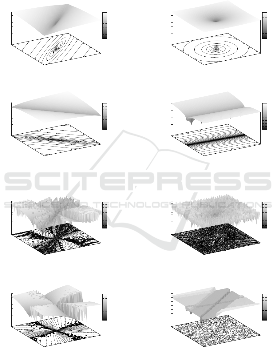
Obviously, characteristics of pcetb(δ) depicted in

Fig. 1 (generated for δ = 0.0001) looks the same

as the characteristics of pctb (see (Trojanowski and

Kulpa, 2015) for comparisons) and have the same dis-

tinctive shape of a funnel. Thus, as in the case of pctb,

they can also be classiﬁed into four main types.

Empirical evaluation of pcet is difﬁcult, so, we in-

troduce the less restrictive measure, that is, a particle

weak convergence time.

Deﬁnition 4.2 (The particle weak convergence ex-

pected time). Let δ be a given positive number. The

particle weak convergence expected time pwcet(δ) is

the minimal number of steps necessary to get the ex-

pected value of difference between subsequent parti-

cle locations lower than δ, that is

pwcet(δ) = min{t : |e

− e

t+1

| < δ}. (26)

It is obvious that pwcet(δ) ≤ pcet(δ) and equality

generally does not hold. Empirical characteristics of

pwcet are depicted in Fig. 2 and Fig. 3. The charac-

teristics were obtained with Algorithm 1.

Algorithm 1 : Particle weak convergence expected time

evaluation procedure.

1: Initialize: T

max

= 1e+5, two successive expected

locations e

and e

, and an attractor of a particle,

for example, y = 0.

2: s

= e

− e

3: f = (c

+ c

)/2

4: t = 1

5: repeat

6: e

t+1

= (1 + w − f )e

− we

t−1

+ f y

7: s

t+1

= e

t+1

− e

8: t = t + 1

9: until (s

> δ) ∧ (s

< 1e+10) ∧(t < T

max

)

10: if s

< 1e+10 then

11: return t

12: else

13: return T

max

14: end if

Fig. 2 depicts the values of pwcet generated for

δ = 0.0001 as a function of initial location and veloc-

ity represented by expected locations e

and e

where

E[φ

] and w are ﬁxed. A grid of pairs [e

] consists

of 40000 points (200 × 200) varying from -10 to 10

for both e

and e

Fig. 3 shows the values of pwcet also for δ =

0.0001 obtained for a grid of conﬁgurations (φ

max

,w)

starting from [φ

max

= 0.0, w = −1.0] and changing

with step 0.02 for w and step 0.04 for φ

max

(which

gave 200 × 100 points).

ECTA 2016 - 8th International Conference on Evolutionary Computation Theory and Applications

-8

-4

-8

-4

100

200

300

400

500

600

E[φ

]=0.06; w=0.96; y=0

250

300

350

400

450

500

550

600

(a) type A

-8

-4

-8

-4

100

200

300

400

500

600

E[φ

]=1.76; w=0.96; y=0

350

400

450

500

550

600

(b) type B

-8

-4

-8

-4

100

200

300

400

500

600

700

E[φ

]=3.91; w=0.96; y=0

350

400

450

500

550

600

650

700

750

-8

-4

-8

-4

200

400

600

800

1000

1200

E[φ

]=2.11; w=0.06; y=0

400

500

600

700

800

900

1000

1100

1200

1300

(d) type D

Figure 1: Graphs of pcetb(e

) for selected conﬁgurations (E[φ

],w).

-10

-5

-10

-5

100

150

200

250

300

350

400

450

500

E[φ

]=0.06; w=0.96; y=0

100

150

200

250

300

350

400

450

500

(a) type A

-10

-5

-10

-5

100

150

200

250

300

350

400

450

500

E[φ

]=1.76; w=0.96; y=0

100

150

200

250

300

350

400

450

500

(b) type B

-10

-5

-10

-5

100

200

300

400

500

600

E[φ

]=3.91; w=0.96; y=0

100

200

300

400

500

600

-10

-5

-10

-5

E[φ

]=2.11; w=0.06; y=0

(d) type D

Figure 2: Graphs of recorded values of pwcet(e

) for selected conﬁgurations (E[φ

],w).

Particle Convergence Expected Time in The PSO Model with Inertia Weight

-1

-0.5

0.5

100

1000

10000

100000

E[φ

]

10000

20000

30000

40000

50000

60000

70000

80000

90000

100000

110000

0 1 2 3 4 5 6 7 8

E[φ

]

-1

-0.5

0.5

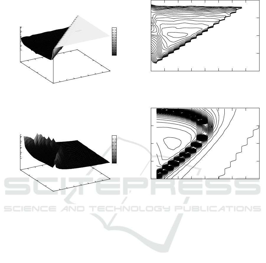
Figure 3: Recorded convergence times of the particle location pwcet(E[φ

],w) for example starting conditions: e

= −9 and

= −5; 3D shape with logarithmic scale for pwcet(E[φ

],w) (left graph), and isolines from 0 to 100 with step 5 (right graph).

-1

-0.5

0.5

100

1000

10000

E[φ

]

2000

4000

6000

8000

10000

12000

14000

16000

0 1 2 3 4 5 6 7 8

E[φ

]

-1

-0.5

0.5

Figure 4: Recorded convergence times of the particle location variance pvwct(E[φ

],w) for example starting conditions:

= −9 and e

= −5; 3D shape with logarithmic scale for pvwct(E[φ

],w) (left graph), and isolines from 0 to 20000 with

step 10 (right graph).

In both ﬁgures the conﬁgurations generating

pwcet > 100000 have assigned a constant value of

100000. It is also assumed that c

= c

= φ

max

/2.

5 CONVERGENCE OF

VARIANCE OF PARTICLE

LOCATION DISTRIBUTION

Convergence of the expected value of the particle lo-

cation still does not guarantee the convergence of the

particle position. This is the case, for example, where

the particle oscillates symmetrically and the oscilla-

tions do not fade. In (Poli, 2009) author studied con-

vergence of the variance and standard deviation of the

particle location and obtained region (Ineq. (3)) of the

order-2 stability of the system. In the studied model

with the best particle stagnation assumption described

by Eq. (6) the variance of the particle location con-

verges to zero for the conﬁgurations originating from

the order-2 stability region (Ineq. 3).

It is interesting to show how fast the variance of

a particle location fades. Formally, we are interested

in evaluation of the particle location variance conver-

gence time. Below, d

denotes variance of particle

location in time t, that is

= Var[x

] = m

− e

. (27)

Deﬁnition 5.1 (The particle location variance con-

vergence time). Let δ be a given positive num-

ber. The particle location variance convergence time

pvct(δ) is the minimal number of steps necessary to

get the variance of particle location lower than δ for

all subsequent time steps, that is

pvct(δ) = min{t : d

< δ f or all s ≥ t}. (28)

Empirical evaluation of pvct is difﬁcult, so, we in-

troduce the less restrictive measure, that is, a particle

location variance weak convergence time.

Deﬁnition 5.2 (The particle location variance weak

convergence time). Let δ be a given positive number.

The particle location variance weak convergence time

pvwct(δ) is the minimal number of steps necessary to

ECTA 2016 - 8th International Conference on Evolutionary Computation Theory and Applications

get the variance of particle location lower than δ, that

pvwct(δ) = min{t : d

< δ}. (29)

As in the case of pwcet(δ) and pwct(δ) it is also

obvious that pvwct(δ) ≤ pvct(δ) and equality gener-

ally does not hold.

When pvwct(δ) has to be calculated according to

Def. 5.2, it is important to select appropriately initial

values of the algorithm parameters: h

and m

. To do

this, lets ﬁrst note that Eq. (1) can be converted to the

form:



t+1

= w · v

+ ϕ

(y − x

t+1

= x

+ v

t+1

(30)

When we substitute zero for t in Eq. (30) we obtain

Eq. (31):

= x

+ w · v

+ ϕ

(y − x

). (31)

Let us assume, that x

and v

are independent ran-

dom variables. Applying the expectation operator to

both sides of Eq. (31) we get

= e

(1 − f ) + w · s

+ f y, (32)

where s

= Ev

. From Eq. (32) we obtain

− e

(1 − f ) − f y

. (33)

Multiplying both sides of Eq. (31) by x

we get

= x

(1 − ϕ

) + wx

+ x

y. (34)

Applying expectation operator to both sides of the

Eq. (34) we obtain

= m

(1 − f ) + we

+ e

f y, (35)

and substituting expression from Eq. (33) for s

= m

(1 − f ) + e

− e

(1 − f ) − f y) + e

f y.

(36)

Eventually, above formula can be simpliﬁed to the

form

= (m

− e

)(1 − f ) + e

, (37)

or equivalent

= d

(1 − f ) + e

. (38)

Next, we raise both sides of Eq. (31) to the second

power and obtain

(1 − ϕ

)

+ w

+ ϕ

+ 2wx

(1 − ϕ

+ 2x

(1 − ϕ

+ 2x

(1 − ϕ

)ϕ

y + 2wv

(39)

Applying the expectation operator to both sides of

Eq.(39) and because of the statistical independence

of x

, ϕ

and v

we get

(1 − 2 f + g) + w

+ gy

+ 2we

(1 − f )s

+ 2e

( f −g)y + 2ws

f y,

(40)

where s

= Ev

. Expression from Eq. (33) can be

substituted for s

in Eq. (40). This way we obtain

(1 − 2 f + g) + w

+ gy

+ 2(e

− e

(1 − f ) − f y)(e

(1 − f ) + f y).

(41)

Let d

= Var[x

] and l

= Var[v

] are given. Then

we can calculate

= e

+ d

and

= s

+ l

what can be written in view of Eq. (33) as

− e

(1 − f ) − f y)

+ l

. (42)

Expression from Eq. (42) can be substituted for s

Eq. (41). This way one can obtain the ﬁnal version of

equation for m

(1 − 2 f + g) + w

+ gy

+ e

− (e

(1 − f ) + f y)

(43)

Algorithm 2: Particle location variance weak convergence

time evaluation procedure.

1: Initialize: T

max

= 1e+5, two successive expected

locations e

and e

, variance of initial location

and velocity, for example, d

= 0 and l

= 1 re-

spectively, and an attractor of a particle, for ex-

ample, y = 0.

2: f = (c

+ c

)/2;

3: g = (c

)

/12 + (c

)

/12 + ((c

+ c

)/2)

;

4: m

= e

+ d

5: m

= m

(1 − 2 f + g) +w

+ gy

+ e

− (e

(1 −

f ) + f y)

6: h

= d

(1 − f ) + e

7: d

= m

− e

8: t = 1

9: repeat

10: h

t+1

= (1 + w − f )m

− wh

+ f ye

11: e

t+1

= (1 + w − f )e

− we

t−1

+ f y

12: m

t+1

= m

((1 + w)

− 2(1 + w) f + g) +

t−1

−2h

w(1+w − f )+2e

y( f (1+w)−g)−

t−1

wy f +y

13: d

t+1

= m

t+1

− e

t+1

14: t = t + 1

15: until (d

> δ) ∧ (d

< 1e+10) ∧(t < T

max

)

16: if d

< 1e+10 then

17: return t

18: else

19: return T

max

20: end if

Particle Convergence Expected Time in The PSO Model with Inertia Weight

-10

-5

-10

-5

300

350

400

450

500

550

E[φ

]=0.06; w=0.96; y=0

300

320

340

360

380

400

420

440

460

(a) type A

-10

-5

-10

-5

300

320

340

360

380

400

420

440

E[φ

]=1.76; w=0.96; y=0

300

320

340

360

380

400

420

440

(b) type B

-10

-5

-10

-5

E[φ

]=3.91; w=0.96; y=0

-10

-5

-10

-5

E[φ

]=2.11; w=0.06; y=0

(d) type D

Figure 5: Graphs of recorded values of the particle location variance pvwct(E[φ

],w) for selected conﬁgurations (E[φ

],w).

Empirical characteristics of the particle location

variance weak convergence time (pvwct) are given in

Fig. 4 and Fig. 5.

As in the case of empirical characteristics of

pwcet, Fig. 4 shows the values of pvwct also ob-

tained for a grid of conﬁgurations (φ

max

,w) start-

ing from [φ

max

= 0.0, w = −1.0] and changing with

step 0.02 but in both directions (which also gave

200 × 100 points). The conﬁgurations generating

pvwct > 100000 also have assigned a constant value

of 100000 and it is assumed that c

= c

= φ

max

/2.

Fig. 5 presents the values of pvwct as a function

of e

and e

where E[φ

] and w are ﬁxed. The grid

of pairs [e

] consists of 40000 points (200 × 200)

varying from -10 to 10 for both e

and e

The characteristics depicted in Fig. 4 and Fig. 5

were obtained with Algorithm 2 for selected values of

variance of initial location d

= 0 and velocity l

= 1.

6 CONCLUSIONS

In the presented research for the stochastic model of

PSO with inertia weight we propose new measures

inspired by the measure of particle convergence time

earlier deﬁned for the deterministic model of PSO.

The proposed measures are based on the order-1 and

order-2 analysis of PSO dynamics.

The order-1 equivalent of particle convergence

time (pct) is the particle convergence expected time

pcet(δ) which represents the minimal number of steps

necessary for the expected particle location to obtain

equilibrium. As in the deterministic case, the upper

bound formula (pcetb(δ)) is also derived.

For the order-2 analysis of the PSO model the par-

ticle location variance convergence time pvct(δ) is

proposed as a minimal number of steps necessary to

get variance of particle location lower than δ for all

subsequent time steps.

Weak versions of pcet(δ) and pvct(δ), that is,

pwcet(δ) and pvwct(δ) are also proposed as more

convenient for experimental evaluation. Empirical

characteristics of pwcet(δ) and pvwct(δ) are pre-

sented. The issue of appropriate selection of initial

parameters for the pvwct(δ) evaluation procedure is

discussed.

ACKNOWLEDGMENTS

The authors would like to thank Prof. Mohammad

Reza Bonyadi for inspiration and valuable comments

and directions.

ECTA 2016 - 8th International Conference on Evolutionary Computation Theory and Applications

REFERENCES

Bonyadi, M. R. and Michalewicz, Z. (2016a). Analysis of

stability, local convergence, and transformation sensi-

tivity of a variant of particle swarm optimization algo-

rithm. IEEE T. Evolut. Comput., 20(3):370–385.

Bonyadi, M. R. and Michalewicz, Z. (2016b). Particle

swarm optimization for single objective continuous

space problems: a review. Evol. Comput. Date of

Publication: March 8, 2016.

Cleghorn, C. W. and Engelbrecht, A. P. (2014). A gener-

alized theoretical deterministic particle swarm model.

Swarm Intelligence, 8(1):35–59.

Cleghorn, C. W. and Engelbrecht, A. P. (2015). Particle

swarm variants: standardized convergence analysis.

Swarm Intelligence, 9(2):177–203.

Jiang, M., Luo, Y. P., and Yang, S. Y. (2007). Stochastic

convergence analysis and parameter selection of the

standard particle swarm optimization algorithm. In-

formation Processing Letters, 102(1):8–16.

Lehre, P. K. and Witt, C. (2013). Finite First Hitting Time

Versus Stochastic Convergence in Particle Swarm Op-

timisation, pages 1–20. Springer New York.

Liu, Q. (2015). Order-2 stability analysis of particle swarm

optimization. Evol. Comput., 23(2):187–216.

Poli, R. (2008a). Analysis of the publications on the appli-

cations of particle swarm optimisation. J. Artif. Evol.

App., 2008:4:1–4:10.

Poli, R. (2008b). Dynamics and stability of the sampling

distribution of particle swarm optimisers via moment

analysis. Journal of Artiﬁcial Evolution and Applica-

tions, 2008(Article ID 761459).

Poli, R. (2009). Mean and variance of the sampling distri-

bution of particle swarm optimizers during stagnation.

IEEE T. Evolut. Comput., 13(4):712–721.

Poli, R. and Broomhead, D. (2007). Exact analysis of the

sampling distribution for the canonical particle swarm

optimiser and its convergence during stagnation. In

GECCO ’07: Proceedings of the 9th annual confer-

ence on Genetic and evolutionary computation, vol-

ume 1, pages 134–141. ACM Press.

Trelea, I. C. (2003). The particle swarm optimization algo-

rithm: convergence analysis and parameter selection.

Inform. Process. Lett., 85(6):317 – 325.

Trojanowski, K. and Kulpa, T. (2015). Particle convergence

time in the PSO model with inertia weight. In Pro-

ceedings of the 7th International Joint Conference on

Computational Intelligence (IJCCI 2015) - Volume 1:

ECTA, pages 122–130.

van den Bergh, F. and Engelbrecht, A. P. (2006). A study of

particle swarm optimization particle trajectories. In-

form. Sciences, 176(8):937–971.

Witt, C. (2009). Why standard particle swarm optimisers

elude a theoretical runtime analysis. In Proceedings of

the Tenth ACM SIGEVO Workshop on Foundations of

Genetic Algorithms, FOGA ’09, pages 13–20. ACM.

Particle Convergence Expected Time in The PSO Model with Inertia Weight