
Pedestrian Trajectory Prediction in Large Infrastructures
A Long-term Approach based on Path Planning
Mario Garz
´
on, David Garz
´
on-Ramos, Antonio Barrientos and Jaime del Cerro
Centro De Autom
´
atica y Rob
´
otica UPM-CSIC,
Calle Jos
´
e Guti
´
errez Abascal, 2, 28006 Madrid, Spain
Keywords:
Pedestrian Trajectory Prediction, Planning-based Prediction, Trajectory Forecast.
Abstract:
This paper presents a pedestrian trajectory prediction technique. Its mail novelty is that it does not require any
previous observation or knowledge of pedestrian trajectories, thus making it useful for autonomous surveil-
lance applications. The prediction requires only a set of possible goals, a map of the scenario and the initial
position of the pedestrian. Then, it uses two different path planing algorithms to find the possible routes and
transforms the similarity between observed and planned routes into probabilities. Finally, it applies a motion
model to obtain a time-stamped predicted trajectory. The system has been used in combination with a pedes-
trian detection and tracking system for real-world tests as well as a simulation software for a large number of
executions.
1 INTRODUCTION
Predicting the future trajectory of a pedestrian in a
given environment is a very useful task for many ap-
plications, both in the robotics world as in social sci-
ences. This work presents a novel approach for this
task, that can be used in any given scenario without
previous observation or data-collection.
This work is focused on a very common appli-
cation of pedestrian trajectory prediction: the au-
tonomous surveillance of critical infrastructures, such
as harbours, power plants or security facilities. Nowa-
days, surveillance systems are mostly static and they
require continuous monitoring by a human. More-
over, they are usually limited to provide reactive in-
formation (e.g. motion sensors, alarms on doors and
windows, etc). Therefore, they require a response
from the users which in some cases may not have
enough time to effectively address the incident. In this
context, predicting the possible goal of a given pedes-
trian, as well as the route and time that will take him
or her to the goal can help to increase the effectiveness
of the surveillance system because the prediction can
provide the ability of responding efficiently and on
time to potential vulnerabilities, such as the presence
or approximation of intruders to restricted or vulnera-
ble locations.
When performing autonomous surveillance of a
critical infrastructure, a series of important or vulner-
able locations can be clearly defined. Moreover, it can
be assumed that an intruder moving on the infrastruc-
ture has a knowledge of the complete map, and there-
fore it can also perform a long-term planning of his or
her own route. Furthermore, the prediction does not
need to be highly accurate, because the objective of
the prediction algorithm will be to find the most prob-
able destination and its route so a robot can be sent to
obtain a detailed image of the intruder. Moreover, in
order to obtain the prediction, only a few requisites,
analogous those required by any path planning algo-
rithm, are needed. Namely: The initial position of the
pedestrian, a map of the scenario and a list of possible
goals.
Once the initial position, and the set of possible
goals are defined, an efficient route to each one of
them can be obtained. Those possible routes depend
on the cost-map and they are the base of the trajectory
prediction. After this, the objective of the prediction
algorithm will be to find the probability of the pedes-
trian following any of the possible trajectories. This
probability can be computed based on the similarity
between the observed trajectory and each one of the
possible routes. The probability distribution, as well
as the prediction output, can be updated every time a
new observation arrives or at a fixed time-step.
For this work, two different planning techniques
are used and compared: Fast Marching Method
(FMM) (Sethian, 1999) and the widely used A Star
Garzón, M., Garzón-Ramos, D., Barrientos, A. and Cerro, J.
Pedestrian Trajectory Prediction in Large Infrastructures - A Long-term Approach based on Path Planning.
DOI: 10.5220/0005983303810389
In Proceedings of the 13th International Conference on Informatics in Control, Automation and Robotics (ICINCO 2016) - Volume 2, pages 381-389
ISBN: 978-989-758-198-4
Copyright
c
2016 by SCITEPRESS – Science and Technology Publications, Lda. All rights reserved
381

Algorithm (A
∗
). Both of them take into account the
map of the scenario and the possible destination of
the pedestrians but differ on the optimal solution ob-
tained due the heuristically component of A
∗
and the
fact that FMM uses only a 4-connected neighbour-
hood to obtain the route.
The main novelty in this work is that is does
not require any previous observation of pedestrian
trajectories to obtain the prediction, and it can be
adapted to any scenario by requiring only a cost-map,
making it useful for security applications where it
is not likely to have previous observations. Further-
more, the prediction presented is integrated with a
previously-developed pedestrian detection and track-
ing algorithm, so it is capable of handling errors or
noisy measurements present in any real-world detec-
tion system. Finally, by integrating a motion model of
the pedestrian, it is possible to obtain a time-stamped
prediction, which is required for its integration with
autonomous surveillance with mobile robots.
2 RELATED WORK
Most of the pedestrian trajectory prediction tech-
niques that have been proposed are focused on obtain-
ing a short-time prediction, mainly for robot naviga-
tion in scenarios where people and robots may found
themselves together.
An early work was based on multi-layer Bayesian
dynamic structures, where each layer represents a
path trough the environment (Bui et al., 2001). A
different work was based on Hidden Markov Models,
using clustering obtained form expectation maximiza-
tion (Bennewitz et al., 2005). However, it requires a
high load of previous observations, it is scenario de-
pendent and it does not consider time or velocities. A
prediction based on genetic algorithms and an agent-
based was tested on a large shopping centre, however,
it does not take into account any time constraint be-
cause it is oriented to recreate trajectories in social
studies (Kitazawa and Batty, 2004).
Some works have proposed to predict the pedes-
trian trajectory using a goal-directed prediction. The
goals may be obtained from clustering large amounts
of observations (Yen et al., 2008) or by topological
places in a map (Ikeda et al., 2012). Then data from
observations was used to obtain probability of transi-
tion between sub-goals. The main drawback of these
works is their dependence on scenario specific infor-
mation and their limitation on time and length of the
prediction.
A two level prediction process has been also pro-
posed (Foka and Trahanias, 2010), it defines a short-
term prediction based on Polynomial Neural Net-
works, and a long-term prediction based on the prob-
ability of transition between a series of manually de-
fined ”Hot Points”. This technique however only di-
rects the future position of the pedestrian and does not
take into account time or velocity issues.
A more recent approach proposes a probabilistic
method of determining pedestrian trajectory (Tamura
et al., 2013). It classifies the behaviours of pedes-
trians into definite patterns, learned through observa-
tion. Then compares a new one by likelihood cal-
culation. This technique however does not take into
account the environment and it only predicts simple
trajectories based on the direction of the movement.
A more complex algorithm models goal-directed
trajectories of pedestrians using maximum entropy in-
verse optimal control (Ziebart et al., 2009). This ap-
proach describes the environment by using generic
features, which then can be moved. Then, it cre-
ates a cost-map based on previously observed trajec-
tories, and uses it to plan a future trajectory of the
newly observed pedestrian. This work was later ex-
tended by adding vision based physical scene features
and noisy tracker observations (Kitani et al., 2012).
Those works are similar to the one proposed in this
paper in the sense that they also use a planning step
to predict the future position of the pedestrian, how-
ever, their long-term prediction is not very clear, be-
cause it only directs its future position and therefore
it is only valid in relatively short distances, further-
more, time or velocity issues are not accounted for,
and as with all other prediction techniques they re-
quire a large amount of observations.
The main novelty of the prediction technique pro-
posed in this paper, is that it does not require any
previous observations of pedestrians in order to ob-
tain the prediction, as does every previous work. This
means that can be used in any scenario, only having
its map. Another difference with previous works is
that the work presented here uses a Kalman filter to
obtain the pedestrian velocity and combines it with
a path planning based prediction. This combination
results in a long-term prediction that can take into ac-
count not only the position but also time and velocity
constraints. Finally, it is possible to obtain predictions
that model the different behaviours of pedestrians by
modifying the cost-map and using different path plan-
ning techniques, therefore increasing the adaptability
of the prediction to any infrastructure or depending on
the user’s necessities.
ICINCO 2016 - 13th International Conference on Informatics in Control, Automation and Robotics
382
3 METHODOLOGY OVERVIEW
As aforementioned, the prediction process has three
inputs: The list of possible goals, the map of the sce-
nario and the pedestrian position. The process is ini-
tialized by defining the first two while the third one
will change continuously as the pedestrian moves.
Moreover, the other two are only processed once at
the initialization of the algorithm and then only if a
re-initialization is executed.
Two independent threads are used, one for pro-
cessing the income data and other for computing the
prediction. Therefore the predicted trajectory can be
produced at a constant frequency, independently from
the rate at which observations are received. Once the
target position is received, it is sent simultaneously to
both the Kalman filter and the prediction process.
When the first position is received an instance of a
Kalman filter is created. Then, every time a new ob-
servation arrives, the filter is updated and a new cycle
of its loop is executed, this allows to keep an accurate
model of the movement of the pedestrian.
The prediction process also receives the initial po-
sition, then it uses a planner (A
∗
or FMM) to obtain
an efficient path from the initial position to each one
of the possible destinations, the initialization is com-
pleted by assigning an equal probability value to each
one of the possible routes. Then, when new observa-
tions arrive, the trajectory followed by the pedestrian
is compared to the possible routes. The result of this
comparison is translated into probabilities so the most
similar route will have the highest probability.
Finally, the long-term prediction is obtained by
projecting the position and velocity observed into the
planned route. The prediction can be as long as the
complete route or according to a given parameter. In
order to account for changes in the direction or un-
predicted movements, the process is restarted if the
pedestrian moves far away from the route or after a
given lapse of time. The complete prediction process
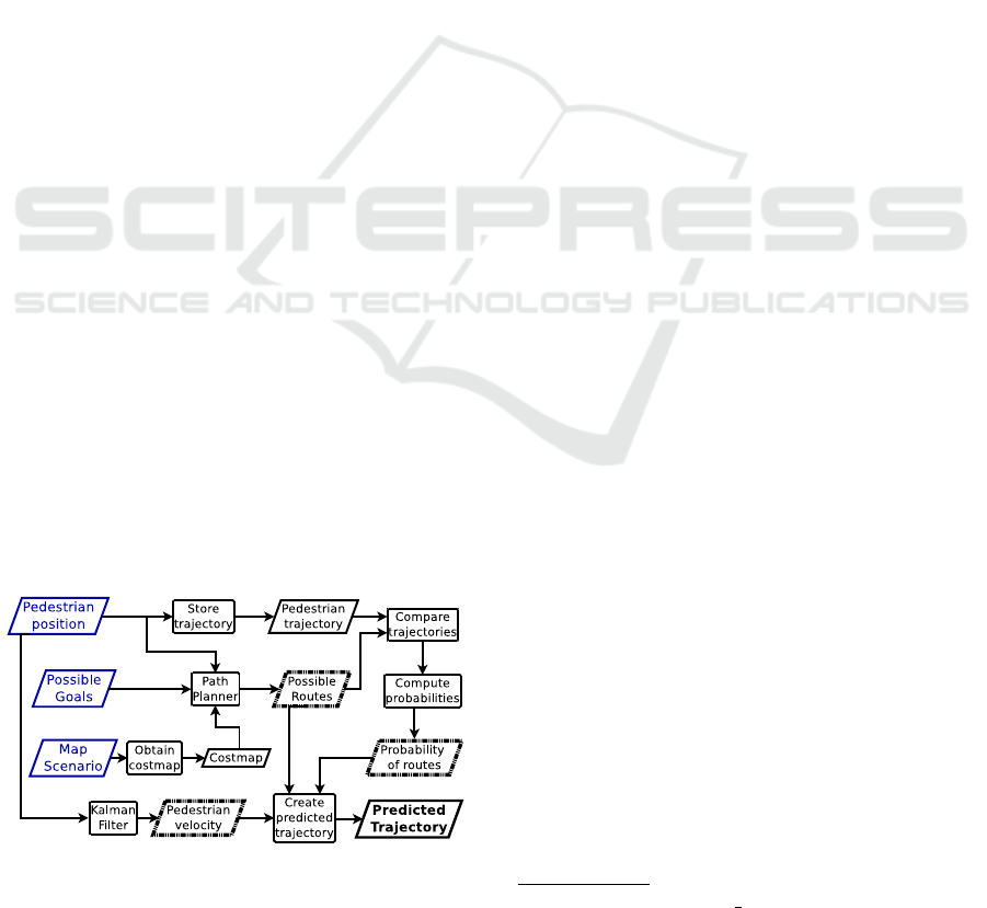
is summarized in Figure 1.
Figure 1: Overview of the proposed approach. The inputs
of the algorithm are shown in blue, the main components,
as well as the trajectory output, are highlighted.
4 TRAJECTORY PREDICTION
BASED ON PATH PLANNING
The core of the prediction algorithm is the use of a
path planning strategy. Its main objective is to obtain
the most likely destination of the pedestrian as well
as its possible trajectory towards it. The problem is
simplified by defining a fixed number of possible des-
tinations, and then compare the observed trajectory of
the pedestrian with the possible routes obtained from
a path planning algorithm. After this, the similarities
are translated into probabilities and the most likely
route is extracted out and considered as the predicted
trajectory. The main components of the algorithm will
be described next.
4.1 Obtaining the Cost-map
The first input to be processed is the map of the sce-
nario, which is used to obtain the cost-map required
for the path planner. This cost-map is of high impor-
tance, because it will determine the behaviour of the
trajectory prediction. Moreover, the process used to
obtain it can be taken as a replacement to the observa-
tions of past pedestrian trajectories required by most
of the prediction algorithms in the literature.
The algorithm uses the standard ROS map format
1
which defines the map in two files: a yaml file which
contains the meta-data and defines the name of the
map image. The second file is the image, which de-
scribes the occupancy state of each cell of the map.
It marks free cells with whiter colours and occupied
ones with black. The map can be obtained from a
SLAM algorithm or it can be created using informa-
tion from a Geographical Information System (GIS).
The first step in processing the map is to scale it
(i.e change its resolution). Maps used in ROS have
usually high resolution because they are used for au-
tonomous navigation (e.g. 0.05m per pixel). How-
ever, a much lower resolution can be used for this
task. Taking into account the frequency of the de-
tection algorithm, the expected mean size of pedes-
trians and the required precision of the algorithm, the
resolution can be much lower, for the presented ex-
periments a value of 0.35m per pixel was defined.
This decrease in resolution will speed up and facili-
tate the complete process, moreover other prediction
techniques also use low resolution maps(Ikeda et al.,
2012). The scaling process is done by using a bilinear
interpolation technique, ensuring that positions in the
resulting map have a correct translation to the original
one. This allows using the result of the prediction in
the original, unscaled, map.
1
http://wiki.ros.org/map server
Pedestrian Trajectory Prediction in Large Infrastructures - A Long-term Approach based on Path Planning
383

The second step in processing the map is to mod-
ify it by incorporating additional obstacles. Those ob-
stacles may represent static objects not included in the
original map, or they can also represent virtual obsta-
cles used to define zones where the pedestrian is not
expected to cross, or to block passages that need to
be avoided. This obstacles can be manually added by
defining its position and radius, or they can be given
as a new map of obstacles that can be added to the
original one.
After the obstacles map is completed, the map is
modified by applying transformations or filters, such
as a distance transformation, median or low pass fil-
ters as well as any other geometrical transformation.
This transformation allows to change the costs in the
surroundings of the obstacles, and therefore modi-
fying the planned routes to common pedestrian be-
haviours (i.e. generate trajectories by the center of
halls, closer to walls, or avoid crossroads or areas
where other pedestrians may be found). This transfor-
mations are applied homogeneously to the complete
map, so it does not include any preference on the pre-
dicted trajectories. An example of the map processing
with an artificial map is presented on Figure 2.
(a) Original map (b) Scaled map
(c) Map with obstacles (d) Resulting Costmap
Figure 2: Steps in the process of obtaining the prediction
cost-map from a given (artificial) map.
4.2 Path Planning for Prediction
Since this work is not focused on developing a new
planning technique, two well known planners (A
∗
and
Fast Marching Method) have been used. However, as
aforementioned, any planner based on a cost-map can
be used. It should be clarified that the implementation
of the path planning algorithms used here does not
take into account the orientation of the pedestrian, nor
it poses any kinematic restriction to its movements.
There are two reasons for this: First, pedestrians can
move in any direction in a plane and second, the de-
tection and tracking algorithm used does not provide
information about the pedestrian orientation.
The planner uses the same three inputs as the com-
plete algorithm: The list of possible goals, which are
defined in map coordinates and can be pre-fixed or
given manually to the algorithm. The second input is
the cost-map, which is received after the pre-process
described in Section 4.1. The third input is the first
position received from the detection algorithm.
Once these inputs are defined, the planner obtains
an effective route from the initial position to each one
of the possible goals in a sequential manner. Each
time a route is found, it is stored and the algorithm re-
mains on stand-by until all possible routes are found.
An example of the result using the A
∗
planner, which
uses the euclidean distance to the goal as heuristic
cost, is depicted on Figure 3.
Figure 3: Possible pedestrian routes (shown in colours)
from an initial position (red rectangle) towards different
possible goals.
4.3 Comparing Two Trajectories
Once the possible routes are defined, the next step is
to compare them with the trajectory that pedestrian
is following so the results can be later translated into
probabilities. There are several issues to take into ac-
count when comparing the trajectories, the first one is
that the possible routes may have different length and
they do not have any time constraints. Also, the dis-
tance should be computed with the information avail-
able at each moment (i.e. the trajectory observed so
far) and it should be updated every time a new obser-
vation arrives.
It was necessary to define a method to measure
the similarity between two trajectories, one that can
be used without requiring time-stamped positions, or
complex computations. The measurement technique
used is based on the Fr
´
echet distance (Fr
´
echet, 1906),
which can be defined as follows: “A man is walking
a dog on a leash: the man can move on one curve,
the dog on the other; both may vary their speed, but
backtracking is not allowed. What is the length of
the shortest leash that is sufficient for traversing both
curves?”(Alt and Godau, 1995).
ICINCO 2016 - 13th International Conference on Informatics in Control, Automation and Robotics
384

The distance computation proposed here also re-
lies on the sum of the point-to-point distance between
each of possible routes. However some differences
are introduced. First of all, since the planned routes
do not have time constraints, and their length can be
different, the minimum distance between each point
in the pedestrian trajectory and the routes is used. An-
other difference is that the distance values are updated
every time a new observation arrives, meaning that
the distance between the trajectories D
tra j
changes ac-
cordingly at every time-step, as defined in Equation
(1).
D
tra j
(n − 1) =
n−1
∑
i=0
d
i
D
tra j
(n) = D
tra j
(n − 1)+ d
n
(1)
Where d
i
represents the distance from the observa-
tion i to the possible route. D
tra j
(n−1) is the distance
up to the n − 1 observation. The complete distance
D
tra j
(n) is obtained by adding the distance from the
last observation to the predicted route d
n
whenever a
new observation is received
4.4 Obtain Likelihood and Probabilities
The next step in the algorithm is to translate the simi-
larities into probabilities. A first approach was to nor-
malize them so the result can be directly translated
to probability values. Taking into account that the
distance value is punctual and defined at each time-
step, the normalization is straightforward. First, the
total distance value D
total
is obtained, by adding the
distance to each one of the possible routes D
j
. Then
the probability of each route P
G
will be the ratio be-
tween each distance and the total distance value, as
expressed by (2).
P
1
=
D
1
D
total
; P
2
=
D
2
D
total
; . . . P
j
=
D
j
D
total
;
(2)
However, after some initial tests, it was found that
using the similarity of all the observed trajectory in-
duce errors, because the pedestrians may not follow
the predicted route, they can change direction or even
go back. In order to solve this, it was necessary to
propose a different computation, one that allows to
give more relevance to the more recent observations
without completely disregarding the previous ones.
The new approach consists on using a memory of
the trajectory observed so far, which will slowly fade
as new observations arrive. To obtain this, a combined
probability with two components is computed. The
first component will be obtained from the last obser-
vation only, and the second one will be the memory of
the previous prediction. This approach has a twofold
advantage, firstly it uses a very simple computation.
Secondly, it allows to control the weight of both cur-
rent and previous values, so as to adapt them to differ-
ent types of behaviours or scenarios. The combined
probability computation is expressed in Equation (3).
P
j
(t) = αP
j
(t − 1) + (1 − α)
ˆ
P
j
(3)
Where P
j
(t) represents the probability of the
pedestrian following any given trajectory P
j
at time
t. And α is the weight factor (0.6 for the experi-
ments) that allows to take into account the previously
observed trajectory, and finally
ˆ
P
j
is the probability
value obtained using only the last observation. This
process is also illustrated in Figure 4.
Figure 4: Current and previous distances from pedestrian
position to possible routes, clearer colours represent the
lower weight of those values in the probability computation.
4.5 Create Predicted Trajectory
After the probability computations, the trajectory
with higher value is selected as the predicted
route/goal. In order to generate the trajectory predic-
tion, it is necessary to take into account not only the
goal but also the velocity of the pedestrian. Further-
more, it should be possible to control the time step
and the temporal scope of the prediction.
This is achieved by projecting the current position
and velocity of the pedestrian, extracted from the state
of the Kalman filter, into the route with the higher
probability. The (x, y) velocity is added to the position
on the path previously found, this results in a new po-
sition that is projected back to the planned route. This
procedure is repeated until the length of the prediction
is achieved, this process is depicted in figure 5.
Although this trajectory may introduce some de-
viation or inaccuracies, its prediction is valid for the
Figure 5: Generation of the predicted trajectory, clear blue
shows the most probable route. The predicted trajectory is
shown with connected purple dots.
Pedestrian Trajectory Prediction in Large Infrastructures - A Long-term Approach based on Path Planning
385

security application, because the objective is not to
collide with the pedestrian but rather be able to reach
it with a mobile robot. Furthermore, changes on di-
rection or variation of velocity can be correctly han-
dled by continuously updating the prediction.
5 EXPERIMENTS AND RESULTS
This section describes the experiments performed to
evaluate the proposed prediction method. Both sim-
ulations and real-world pedestrian trajectories have
been tested. First, the scenario and common features
for both experiments are described. Then, the acqui-
sition of simulated and real trajectories is explained,
along with the performance of the prediction system
in every case.
5.1 Scenario
The same scenario was used in both simulated and
real experiments. The location is a real street inter-
section with many obstacles and possible routes for
pedestrian motion. The 2D map was pre-built using
SLAM algorithms. Then, the cost-map was generated
from the map, as described in Section 4.1, and it was
used for getting the predicted routes in simulated and
real-world tests. The original scenario, the map re-
construction as well as the cost-map and the possible
goals are shown in Figure 6.
5.2 Simulations
The pre-built map and a mobile robot, acting as simu-
(a) Aerial view (b) SLAM map
(c) Cost-map (d) Possible goals
Figure 6: Scenario for simulations and real world tests.
lated pedestrian, were loaded in Stage simulator. Five
positions, according to their proximity to important
locations or exits, were selected as possible goals (See
Figure 6(d)). Then, the trajectories were obtained by
teleoperating the pedestrian from one possible goal
to each one of the other four. In all cases the opera-
tor knew the map of the infrastructure and choose the
route for the simulated pedestrian, thus resulting in ar-
bitrary suboptimal routes. This process was repeated
five times for each possible combination, resulting on
a total of 100 recorded trajectories. Finally, the A
∗
and Fast Marching planners to generate the predicted
routes, and the prediction algorithm was applied, re-
sulting in a total of 200 simulations.
This amount of registers allows obtaining valid
information about the efficiency of the prediction
methodology as well as its behaviour when it is used
in conjunction with the A
∗
or the FMM planner.
Three parameters were studied to validate the results:
the number of changes in the most probable route over
the time, the percentage of trajectory covered before
finding the correct route/goal and the percentage of
trajectory covered before the probability of the correct
route reaches 0.5. Moreover, the mean and standard
deviation were calculated for all parameters named
above. The results for the complete data are shown
in Table 1.
Table 1: Results for trajectory prediction. A changes in the
most probable route; B Trajectory covered (%) before find-
ing the correct route/goal; C Trajectory covered (%) before
probability of route reaches 0.5.
A
∗
Planner FMM Planner
µ σ µ σ
A 4.93 2.79 3.01 1.64
B 51.81% 18.58% 50.46% 18.71%
C 61.61% 13.91% 58.39% 16.27%
It was found that the A
∗
planner have more
changes selecting the most probable route over the
time. This fact was associated to the heuristic com-
ponent of this technique. The euclidean distance min-
imization derives in early differentiation of the possi-
ble routes to reach every goal, which causes that ran-
domly movements of the pedestrian have high impact
in the probability distribution since the first time of
the displacement. On the other hand, due to the shared
starting point for the FMM plans, they tend to follow
the same routes for a considerable percentage of the
displacement, resulting in a more stable probability
distribution.
In both cases, the percentage of trajectory covered
before finding the correct route and the percentage be-
fore its probability reaches 0.5 is nearly 50%. This
ICINCO 2016 - 13th International Conference on Informatics in Control, Automation and Robotics
386

value is related to the goals positions in the map (Fig-
ure 6(d)). Several plans go through the intersection at
the centre of the scenario before they split into very
distinct paths. It can be said that this result is strongly
dependent on the map and for that reason this is not
significant to determinate the speed of achieving a
definitive prediction. However, it gives relevant qual-
itative information about high interest positions in the
scenario.
5.3 Real World Experiments
As aforementioned, in order to use the prediction al-
gorithm, it is necessary to have the pedestrian position
in a given map. This was achieved by using a previous
work, where pedestrians are detected by fusing infor-
mation of a camera and a laser scanner, and their po-
sition on a map is given by a tracking algorithm run-
ning on-board a mobile robot (Garz
´
on et al., 2015).
An image of the detection and tracking algorithm and
the corresponding position in the map is presented on
Figure 7.
Figure 7: Screen capture of the pedestrian detection and
tracking algorithm and the corresponding position on the
map.
Several experiments, having similar start and end
points as with the simulations were carried out. The
prediction algorithm was executed on-board the mo-
bile robot, thus testing the real-time capabilities of the
implementation, and the observed results were consis-
tent to those of the simulations.
The behaviour of prediction based on the A
∗
plan-
ner algorithm could be observed in Figure 8(b) where
the most probable route changes several times due to
unexpected variations in the direction of the pedes-
trian at the intersection, as can be seen in Figure 8(a).
The results for the prediction based on the FMM
algorithm were also consistent with the simulations,
the number of changes in the predicted route is lower
because the possible routes share the same path for a
longer period. This can be seen in Figures 9(b) and
9(a) respectively.
In order to compare the proposed prediction with
previous works, the Modified Hausdorff Distance
(a) Possible routes and
pedestrian trajectory
Displacement(m)
0 5 10 15 20 25 30
Probability
0
0.2
0.4
0.6
0.8
1
Route 1
Route 2
Route 3
Route 4
(b) Probabilities evolution
Figure 8: Real experiments using A
∗
Planner.
(a) Possible routes and
pedestrian trajectory
Displacement(m)
0 5 10 15 20 25 30
Probability
0
0.2
0.4
0.6
0.8
1
Route 1
Route 2
Route 3
Route 4
(b) Probabilities evolution
Figure 9: Real experiments using FMM Planner.
(MHD) can be computed. This measurement provides
a standardized a-posteriori information about the sim-
ilarity of the predicted routes and the trajectory fol-
lowed by the pedestrian. Figure 10 shows the evo-
lution of the MHD for the prediction using A
∗
and
FMM, which has an analogous behaviour as that of
the prediction, which was expected because of the
probability computation process is based on compar-
ing distances.
A comparison with previous works can not be di-
rectly performed, because they provide their results in
pixels, not it meters as is done here. However, a rel-
ative estimation could be calculated based on the dif-
ference between maximum and minimum MHD. The
work of (Kitani et al., 2012) has a relative reduction
of 75% and in the results presented here, this relative
reduction is 86%. Although this is not conclusive, it
shows that the proposed technique produces a useful
prediction, even when working in large scenarios.
6 CONCLUSIONS
An approach for pedestrian trajectory prediction was
presented. The proposed methodology, as well as the
experiments and results obtained show that it is pos-
Pedestrian Trajectory Prediction in Large Infrastructures - A Long-term Approach based on Path Planning
387

0 10% 20% 30% 40% 50% 60% 70% 80% 90% 100%
0
1
2
3
4
5
6
7
8
9
Observations Available
Modified Hausdorff Distance (MHD)
A Star
FMM
Figure 10: Modified Hausdorff Distance evolution with the
observations available for A
∗
and FMM planners.
sible to model the approximate behaviour of pedestri-
ans based on using path planning techniques.
The tests have shown that a valid pedestrian tra-
jectory prediction can be obtained without requiring
a large set of previously observed trajectories. This
allows to use the proposed algorithm in any scenario,
requiring only a map and a list of possible goals.
The prediction algorithm was successfully inte-
grated with a pedestrian detection system and it was
executed on-board a mobile robotic platform, thus
validating its capabilities of working in real-time in
both simulations and real-world applications.
Two different path planning algorithms (A
∗
and
FMM) were implemented and tested for prediction.
It was shown that the prediction based on the A
∗
plan-
ner is more prone to be affected by variations in the
movement of the pedestrian, whereas the FMM based
prediction is more stable in this sense. Moreover, it
can be concluded that in terms of the length of the tra-
jectory required to determine the correct route, both
planning techniques produce a similar result, requir-
ing about 50% of the trajectory, although this results
are may be conditioned by the test scenario.
Furthermore, it was possible to use a simple mo-
tion model, based on a Kalman filter to estimate the
time it will take to reach any given goal, thus mak-
ing the time-stamped prediction very useful for any
autonomous surveillance system.
This work has two main lines for future work, the
first one is to try to autonomously find the possible
destinations and the second is to provide a map or set
of maps of predictions where the or different possibil-
ities, uncertainties or variances of the prediction can
be expressed in a better way.
ACKNOWLEDGEMENTS
This work was partially supported by the Robotics
and Cybernetics Group at Universidad Polit
´
ecnica de
Madrid (Spain), and it was funded under the projects:
PRIC (Protecci
´
on Robotizada de Infraestructuras
Cr
´
ıticas; DPI2014-56985-R), sponsored by the Span-
ish Ministry of Economy and Competitiveness and
RoboCity2030-III-CM (Rob
´
otica aplicada a la mejora
de la calidad de vida de los ciudadanos. fase III;
S2013/MIT-2748), funded by Programas de Activi-
dades I+D en la Comunidad de Madrid and co-funded
by Structural Founds of the EU.
REFERENCES
Alt, H. and Godau, M. (1995). Computing the fr
´
echet dis-
tance between two polygonal curves. International
Journal of Computational Geometry & Applications,
5(01n02):75–91.
Bennewitz, M., Burgard, W., Cielniak, G., and Thrun, S.
(2005). Learning motion patterns of people for com-
pliant robot motion. The International Journal of
Robotics Research, 24(1):31–48.
Bui, H. H., Venkatesh, S., and West, G. (2001). Tracking
and surveillance in wide-area spatial environments us-
ing the abstract hidden markov model. International
Journal of Pattern Recognition and Artificial Intelli-
gence, 15(01):177–196.
Foka, A. and Trahanias, P. (2010). Probabilistic au-
tonomous robot navigation in dynamic environments
with human motion prediction. International Journal
of Social Robotics, 2(1):79–94.
Fr
´
echet, M. M. (1906). Sur quelques points du calcul
fonctionnel. Rendiconti del Circolo Matematico di
Palermo (1884-1940), 22(1):1–72.
Garz
´
on, M. A., Barrientos, A., Cerro, J. D., Alacid, A., Fo-
tiadis, E., Rodr
´
ıguez-Canosa, G. R., and Wang, B.-C.
(2015). Tracking and following pedestrian trajecto-
ries, an approach for autonomous surveillance of criti-
cal infrastructures. Industrial Robot: An International
Journal, 42(5):429–440.
Ikeda, T., Chigodo, Y., Rea, D., Zanlungo, F., Shiomi, M.,
and Kanda, T. (2012). Modeling and prediction of
pedestrian behavior based on the sub-goal concept. In
Proceedings of Robotics: Science and Systems, Syd-
ney, Australia.
Kitani, K. M., Ziebart, B. D., Bagnell, J. A., and Hebert, M.
(2012). Computer Vision – ECCV 2012: 12th Euro-
pean Conference on Computer Vision, Florence, Italy,
October 7-13, 2012, Proceedings, Part IV, chapter
Activity Forecasting, pages 201–214. Springer Berlin
Heidelberg, Berlin, Heidelberg.
Kitazawa, K. and Batty, M. (2004). Pedestrian behaviour
modelling. In Developments in Design and Decision
Support Systems in Architecture and Urban Planning,
pages 111–126.
Sethian, J. A. (1999). Fast marching methods. SIAM Re-
view, 41(2):199–235.
Tamura, Y., Terada, Y., Yamashita, A., and Asama, H.
(2013). Modelling behaviour patterns of pedestrians
for mobile robot trajectory generation. International
Journal of Advanced Robotic Systems, 10(301):1–11.
ICINCO 2016 - 13th International Conference on Informatics in Control, Automation and Robotics
388

Yen, H. C., Huang, H. P., and Chung, S. Y. (2008). Goal-
directed pedestrian model for long-term motion pre-
diction with application to robot motion planning.
In Advanced robotics and Its Social Impacts, 2008.
ARSO 2008. IEEE Workshop on, pages 1–6.
Ziebart, B., Ratliff, N., Gallagher, G., Mertz, C., Peterson,
K., Bagnell, J., Hebert, M., Dey, A., and Srinivasa,
S. (2009). Planning-based prediction for pedestrians.
In Intelligent Robots and Systems, 2009. IROS 2009.
IEEE/RSJ International Conference on, pages 3931–
3936.
Pedestrian Trajectory Prediction in Large Infrastructures - A Long-term Approach based on Path Planning
389
